Markov Decision Processes and Exact Solution Methods: Value - PowerPoint PPT Presentation
Markov Decision Processes and Exact Solution Methods: Value Iteration Policy Iteration Linear Programming Pieter Abbeel UC Berkeley EECS Markov Decision Process Assumption: agent gets to observe the state [Drawing from Sutton and Barto,
Markov Decision Processes and Exact Solution Methods: Value Iteration Policy Iteration Linear Programming Pieter Abbeel UC Berkeley EECS
Markov Decision Process Assumption: agent gets to observe the state [Drawing from Sutton and Barto, Reinforcement Learning: An Introduction, 1998]
Markov Decision Process (S, A, T, R, H) Given S: set of states n A: set of actions n T: S x A x S x {0,1,…,H} à [0,1], T t (s,a,s’) = P( s t+1 = s’ | s t = s, a t =a) n R: S x A x S x {0, 1, …, H} à < R t (s,a,s’) = reward for ( s t+1 = s’, s t = s, a t =a) n H: horizon over which the agent will act n Goal: Find ¼ : S x {0, 1, …, H} à A that maximizes expected sum of rewards, i.e., n
Examples MDP (S, A, T, R, H), goal: q Cleaning robot q Walking robot q Pole balancing q Games: tetris, backgammon q Server management q Shortest path problems q Model for animals, people
Canonical Example: Grid World § The agent lives in a grid § Walls block the agent’s path § The agent’s actions do not always go as planned: § 80% of the time, the action North takes the agent North (if there is no wall there) § 10% of the time, North takes the agent West; 10% East § If there is a wall in the direction the agent would have been taken, the agent stays put § Big rewards come at the end
Solving MDPs n In an MDP, we want an optimal policy π *: S x 0:H → A n A policy π gives an action for each state for each time t=5=H t=4 t=3 t=2 t=1 t=0 n An optimal policy maximizes expected sum of rewards Contrast: In deterministic, want an optimal plan, or sequence of actions, n from start to a goal
Outline n Optimal Control = given an MDP (S, A, T, R, ° , H) find the optimal policy ¼ * n Exact Methods: n Value Iteration n Policy Iteration n Linear Programming For now: discrete state-action spaces as they are simpler to get the main concepts across. Will consider continuous spaces later!
Value Iteration n Algorithm: n Start with for all s. n For i=1, … , H Given V i *, calculate for all states s 2 S: n This is called a value update or Bellman update/back-up n = the expected sum of rewards accumulated when starting from state s and acting optimally for a horizon of i steps
Value Iteration in Gridworld noise = 0.2, ° =0.9, two terminal states with R = +1 and -1
Value Iteration in Gridworld noise = 0.2, ° =0.9, two terminal states with R = +1 and -1
Value Iteration in Gridworld noise = 0.2, ° =0.9, two terminal states with R = +1 and -1
Value Iteration in Gridworld noise = 0.2, ° =0.9, two terminal states with R = +1 and -1
Value Iteration in Gridworld noise = 0.2, ° =0.9, two terminal states with R = +1 and -1
Value Iteration in Gridworld noise = 0.2, ° =0.9, two terminal states with R = +1 and -1
Value Iteration in Gridworld noise = 0.2, ° =0.9, two terminal states with R = +1 and -1
Exercise 1: Effect of discount, noise (a) Prefer the close exit (+1), risking the cliff (-10) (1) ° = 0.1, noise = 0.5 (b) Prefer the close exit (+1), but avoiding the cliff (-10) (2) ° = 0.99, noise = 0 (c) Prefer the distant exit (+10), risking the cliff (-10) (3) ° = 0.99, noise = 0.5 (d) Prefer the distant exit (+10), avoiding the cliff (-10) (4) ° = 0.1, noise = 0
Exercise 1 Solution (a) Prefer close exit (+1), risking the cliff (-10) --- ° = 0.1, noise = 0
Exercise 1 Solution (b) Prefer close exit (+1), avoiding the cliff (-10) -- ° = 0.1, noise = 0.5
Exercise 1 Solution (c) Prefer distant exit (+1), risking the cliff (-10) -- ° = 0.99, noise = 0
Exercise 1 Solution (d) Prefer distant exit (+1), avoid the cliff (-10) -- ° = 0.99, noise = 0.5
Value Iteration Convergence Theorem. Value iteration converges. At convergence, we have found the optimal value function V* for the discounted infinite horizon problem, which satisfies the Bellman equations § Now we know how to act for infinite horizon with discounted rewards! § Run value iteration till convergence. § This produces V*, which in turn tells us how to act, namely following: § Note: the infinite horizon optimal policy is stationary, i.e., the optimal action at a state s is the same action at all times. (Efficient to store!) 25
Convergence and Contractions n Define the max-norm: n Theorem: For any two approximations U and V n I.e. any distinct approximations must get closer to each other, so, in particular, any approximation must get closer to the true U and value iteration converges to a unique, stable, optimal solution n Theorem: n I.e. once the change in our approximation is small, it must also be close to correct 26
Outline n Optimal Control = given an MDP (S, A, T, R, ° , H) find the optimal policy ¼ * n Exact Methods: n Value Iteration n Policy Iteration n Linear Programming For now: discrete state-action spaces as they are simpler to get the main concepts across. Will consider continuous spaces later!
Policy Evaluation n Recall value iteration iterates: n Policy evaluation: n At convergence:
Exercise 2
Policy Iteration n Alternative approach: n Step 1: Policy evaluation: calculate utilities for some fixed policy (not optimal utilities!) until convergence n Step 2: Policy improvement: update policy using one- step look-ahead with resulting converged (but not optimal!) utilities as future values n Repeat steps until policy converges n This is policy iteration n It’s still optimal! n Can converge faster under some conditions
Policy Evaluation Revisited n Idea 1: modify Bellman updates n Idea 2: it ’ s just a linear system, solve with Matlab (or whatever), variables: V ¼ (s), constants: T, R
Policy Iteration Guarantees Policy Iteration iterates over: Theorem. Policy iteration is guaranteed to converge and at convergence, the current policy and its value function are the optimal policy and the optimal value function! Proof sketch: (1) Guarantee to converge : In every step the policy improves. This means that a given policy can be encountered at most once. This means that after we have iterated as many times as there are different policies, i.e., (number actions) (number states) , we must be done and hence have converged. (2) Optimal at convergence : by definition of convergence, at convergence ¼ k +1 (s) = ¼ k (s) for all states s. This means Hence satisfies the Bellman equation, which means is equal to the optimal value function V*. 34
Outline n Optimal Control = given an MDP (S, A, T, R, ° , H) find the optimal policy ¼ * n Exact Methods: n Value Iteration n Policy Iteration n Linear Programming For now: discrete state-action spaces as they are simpler to get the main concepts across. Will consider continuous spaces later!
Infinite Horizon Linear Program n Recall, at value iteration convergence we have n LP formulation to find V * : µ 0 is a probability distribution over S, with µ 0 (s)> 0 for all s 2 S. Theorem. V * is the solution to the above LP .
Theorem Proof
Dual Linear Program n Interpretation: n n Equation 2: ensures ¸ has the above meaning n Equation 1: maximize expected discounted sum of rewards n Optimal policy:
Outline n Optimal Control = given an MDP (S, A, T, R, ° , H) find the optimal policy ¼ * n Exact Methods: n Value Iteration n Policy Iteration n Linear Programming For now: discrete state-action spaces as they are simpler to get the main concepts across. Will consider continuous spaces later!
Today and forthcoming lectures Optimal control: provides general computational approach to tackle control n problems. n Dynamic programming / Value iteration n Exact methods on discrete state spaces (DONE!) n Discretization of continuous state spaces n Function approximation n Linear systems n LQR n Extensions to nonlinear settings: n Local linearization n Differential dynamic programming n Optimal Control through Nonlinear Optimization n Open-loop n Model Predictive Control n Examples:
Recommend
More recommend
Explore More Topics
Stay informed with curated content and fresh updates.
