Lecture 1: Introduction Statistical and Computational Methods for - - PowerPoint PPT Presentation

▶

Nov 17, 2023 279 likes •480 views

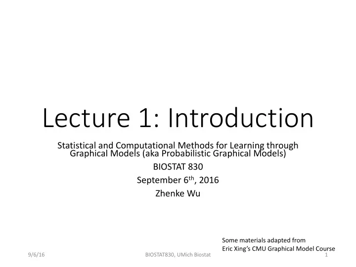
Lecture 1: Introduction Statistical and Computational Methods for Learning through Graphical Models (aka Probabilistic Graphical Models) BIOSTAT 830 September 6 th , 2016 Zhenke Wu Some materials adapted from Eric Xings CMU Graphical Model

SLIDE 1

Lecture 1: Introduction

Statistical and Computational Methods for Learning through Graphical Models (aka Probabilistic Graphical Models) BIOSTAT 830 September 6th, 2016 Zhenke Wu

9/6/16 BIOSTAT830, UMich Biostat 1

Some materials adapted from Eric Xing’s CMU Graphical Model Course

SLIDE 2

Welcome

Course website (Syllabus and notes are posted

here)

http://zhenkewu.com/teaching/graphical_model
Your instructor:
Zhenke Wu PhD, Assistant Professor of Biostatistics
Office Hours:
Tuesday 2-3pm and by appointment
Contact
Instructor: zhenkewu@umich.edu
Class Announcement Email: BIOSTAT-830-001-FA2016-

A@courses.umich.edu

9/6/16 BIOSTAT830, UMich Biostat 2

SLIDE 3

Logistics

Homework Assignment - 30%. (Theory and Implementation)
The total homework grade equals the sum of 3 highest scores out of four, each

corresponding to one learning module and graded in the scale of 0-10.)

The homework will be assigned one week prior to the end of each module.
Assignments will be due 1 week after the module completion.
Active participation - 10%.
Peer-review.
Help oneself learn and teach one’s classmates and instructor by asking questions and

discussing solutions.

Term Project – 60% (Application to your area, or theory/methods work)
(Poster presentation on December 13th, 2016)
Based on the trimmed mean of the scores obtained from external judges and the instructor.
A separate, but optional report will be due at 11:59pm December 20th, 2016.
Students with ONLY poster presentation will be graded solely on poster scores; those with

ADDITIONAL written report will be graded based on the LARGER of the two: the poster and the written report scores.

9/6/16 BIOSTAT830, UMich Biostat 3

SLIDE 4

Course Objectives

To familiarize students with the concepts, applications

and computational techniques of graphical models.

To engage students in building, estimating and

interpreting expert systems for problems either suggested by the instructor or identified by the students.

To showcase the current frontier of graphical model

research in biomedical problems and to prepare advanced PhD or Masters students for their next research projects.

9/6/16 BIOSTAT830, UMich Biostat 4

SLIDE 5

Discussion

What is a statistical model?
Why model?
What is science?
How does statistics, in particular, statistical models

function in scientific investigation?

9/6/16 BIOSTAT830, UMich Biostat 5

SLIDE 6

Reasoning under Uncertainty

9/6/16 BIOSTAT830, UMich Biostat 6

SLIDE 7

Key Questions to be addressed in This Class

Graphical representation of probability

distributions

Inference of model parameters given evidence

from observed nodes

Learn graph structures that are compatible with

data at hand

Use the graphical models for decision making

9/6/16 BIOSTAT830, UMich Biostat 7

SLIDE 8

Brief History of Graphical Models

Represent the interactions between variables using a graph

structure

Statistical physics (Gibbs, 1902, for interacting particles)
Genetics (Wright, 1921, for path analysis on inheritance in natural

species); Largely rejected by statisticians at the time

Economists and social scientists (Wold 1954, Blalock, Jr. 1971)
Statistics (!) (Bartlett, 1935, for contingency tables, or log-linear

models); More accepted thereafter

1960s~70s: Artificial intelligence (AI); Expert systems for locating
il-well, or making medical diagnosis; Great performance with

constrained probabilistic model structure

Late 1980s: widespread acceptance of probabilistic methods

(Theory: Pearl 1988, Lauritzen and Spiegelhalter 1988; Application: Pathfinder expert system by Heckerman et al 1992)

9/6/16 BIOSTAT830, UMich Biostat 8

SLIDE 9

Probabilistic Graphical Models

Connects graph structure with probability

distributions

Advantages:
A general reasoning framework under uncertainty
Interpretability and ease of communication (hence many

scientific applications)

Conditional independence that constrains the model

space

Data integration/fusion
Unobserved/latent variables, missing data easily

handled

9/6/16 BIOSTAT830, UMich Biostat 9

SLIDE 10

Directed Acyclic Graphs (DAG)

Directed edges + nodes gives causality relationships

(Bayesian network)

Generative process

9/6/16 BIOSTAT830, UMich Biostat 10

SLIDE 11

Hidden Markov Model: Speech Recognition

9/6/16 BIOSTAT830, UMich Biostat 11

SLIDE 12

Image Segmentation

9/6/16 BIOSTAT830, UMich Biostat 12

SLIDE 13

DAG for Medical Diagnosis

9/6/16 BIOSTAT830, UMich Biostat 13

SLIDE 14

Undirected Graphs

A node is conditionally independent of every other

node in the graph given its immediate neighbors

Gives correlations; no explicit generative process
Example: solid state physics; Potts model with 4

states on a 2D lattice

9/6/16 BIOSTAT830, UMich Biostat 14

SLIDE 15

Inference Given Observed Evidence in a DAG

Are the nodes “sprinkler” and “rain” correlated if

we see the ground is wet?

“Wet” is a collider
Conditioning on a collider or

its descendants tend to induce dependence among the collider’s parental nodes. (cf. Pg17, Pearl, 2009)

9/6/16 BIOSTAT830, UMich Biostat 15

SLIDE 16

General Inference Questions and Procedures

Inference questions:
Is node X independent of Y given observed node Z?
What is the probability of X=Tail if (Y=Head and

Z=Head)?

What is the joint distribution of (X,Y) given Z?
What is the likelihood of a configuration of node values?
What is the most likely configuration to all or a subset of

the graph?

Computational Procedures
Exact algorithms: junction tree, etc.
Approximate algorithms: variational inference, Monte

Carlo, loopy belief propagation, etc.

9/6/16 BIOSTAT830, UMich Biostat 16

SLIDE 17

Plan for the Class

Module 1 (3 weeks): Representation
1. Graph structure and terminologies; Why study graphical models?
2. Directed graphical models
3. Undirected graphs models
4. Other variants of graphical models
Module 2 (4 weeks): Inference and Computation for Graphical Models
1. Exact and Approximate algorithms
3. Scalable Bayesian algorithms
4. Structure learning
5. Software packages
Module 3 (3 weeks): Graphical Models for Causality
1. Causal graphical models: concepts and inference
2. Structure learning of causal graphs
3. Causal inference for network data (randomization; peer-encouragement design, etc.)
Module 4 (4 weeks): Case Studies
1. Individualized health problems (partially-latent class models, dynamic Bayesian networks, etc.)
2. Large-scale networks (latent state space models)
3. Deep learning examples
4. Graphical models for neuroimaging data (Guest lectures, TBD)
Optional Advanced Topics

9/6/16 BIOSTAT830, UMich Biostat 17

SLIDE 18

Readings for the First Week

Required
Chapters 1-3, Koller and Friedman (2009)
Spiegelhalter, David J., et al. "Bayesian analysis in

expert systems." Statistical science (1993): 219-247.

No pen-and-paper homework assignment for the

first week.

9/6/16 BIOSTAT830, UMich Biostat 18