Introduction to Machine Learning Linear Regression Models Learning - PowerPoint PPT Presentation

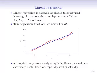
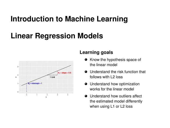
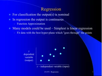
Introduction to Machine Learning Linear Regression Models Learning goals Know the hypothesis space of the linear model 3 Understand the risk function that θ 1 = slope = 0.5 θ 1 = slope = 0.5 2 follows with L2 loss 1 Unit 1 Unit y θ 0 = intercept = 1 θ 0 = intercept = 1 Understand how optimization 1 works for the linear model 0 0 1 2 3 4 Understand how outliers affect x the estimated model differently when using L1 or L2 loss

LINEAR REGRESSION: HYPOTHESIS SPACE We want to predict a numerical target variable by a linear transformation of the features x ∈ R p . So with θ ∈ R p this mapping can be written as: y = f ( x ) = θ 0 + θ T x = θ 0 + θ 1 x 1 + · · · + θ p x p This defines the hypothesis space H as the set of all linear functions in θ : H = { θ 0 + θ T x | ( θ 0 , θ ) ∈ R p + 1 } � c Introduction to Machine Learning – 1 / 16

LINEAR REGRESSION: HYPOTHESIS SPACE 3 θ 1 = slope = 0.5 θ 1 = slope = 0.5 2 1 Unit 1 Unit y θ 0 = intercept = 1 θ 0 = intercept = 1 1 0 0 1 2 3 4 x y = θ 0 + θ · x � c Introduction to Machine Learning – 2 / 16

LINEAR REGRESSION: HYPOTHESIS SPACE Given observed labeled data D , how to find ( θ 0 , θ ) ? This is learning or parameter estimation, the learner does exactly this by empirical risk minimization . NB: We assume from now on that θ 0 is included in θ . � c Introduction to Machine Learning – 3 / 16

LINEAR REGRESSION: RISK We could measure training error as the sum of squared prediction errors (SSE). This is the risk that corresponds to L2 loss : n n y ( i ) − θ T x ( i ) � 2 � � x ( i ) | θ �� � � � y ( i ) , f R emp ( θ ) = SSE( θ ) = = L i = 1 i = 1 1 0 y −1 1 2 3 4 5 6 x Minimizing the squared error is computationally much simpler than minimizing the absolute differences ( L1 loss ). � c Introduction to Machine Learning – 4 / 16

LINEAR MODEL: OPTIMIZATION We want to find the parameters θ of the linear model, i.e., an element of the hypothesis space H that fits the data optimally. So we evaluate different candidates for θ . A first (random) try yields a rather large SSE: ( Evaluation ). 6 θ = ( 1.8 , 0.3 ) 4 2 0 SSE: 16.85 −2 0 2 4 6 8 � c Introduction to Machine Learning – 5 / 16

LINEAR MODEL: OPTIMIZATION We want to find the parameters θ of the linear model, i.e., an element of the hypothesis space H that fits the data optimally. So we evaluate different candidates for θ . Another line yields an even bigger SSE ( Evaluation ). Therefore, this one is even worse in terms of empirical risk. 6 6 θ = ( 1.8 , 0.3 ) θ = ( 1 , 0.1 ) 4 4 2 2 0 0 SSE: 16.85 SSE: 24.3 −2 −2 0 2 4 6 8 0 2 4 6 8 � c Introduction to Machine Learning – 6 / 16

LINEAR MODEL: OPTIMIZATION We want to find the parameters θ of the linear model, i.e., an element of the hypothesis space H that fits the data optimally. So we evaluate different candidates for θ . Another line yields an even bigger SSE ( Evaluation ). Therefore, this one is even worse in terms of empirical risk. Let’s try again: 6 6 6 θ = ( 1.8 , 0.3 ) θ = ( 1 , 0.1 ) θ = ( 0.5 , 0.8 ) 4 4 4 2 2 2 0 0 0 SSE: 16.85 SSE: 24.3 SSE: 10.61 −2 −2 −2 0 2 4 6 8 0 2 4 6 8 0 2 4 6 8 � c Introduction to Machine Learning – 7 / 16

LINEAR MODEL: OPTIMIZATION Since every θ results in a specific value of R emp ( θ ) , and we try to find arg min θ R emp ( θ ) , let’s look at what we have so far: 6 θ = ( 1.8 , 0.3 ) 6 θ = ( 0.5 , 0.8 ) 4 4 2 2 100 0 0 SSE: 16.85 SSE: 10.61 −2 −2 80 0 2 4 6 8 0 2 4 6 8 S S 60 E 40 20 6 θ = ( 1 , 0.1 ) 2 0.0 1 4 0.5 I n 0 2 t e r c Slope e p 1.0 0 −1 SSE: 24.3 t −2 −2 1.5 0 2 4 6 8 � c Introduction to Machine Learning – 8 / 16

LINEAR MODEL: OPTIMIZATION Instead of guessing, we use optimization to find the best θ : 100 80 SSE 60 40 20 2 0.0 1 Intercept 0.5 0 e p 1.0 o −1 l S −2 1.5 � c Introduction to Machine Learning – 9 / 16

LINEAR MODEL: OPTIMIZATION Instead of guessing, we use optimization to find the best θ : 100 80 SSE 60 40 20 2 0.0 1 Intercept 0.5 0 e p 1.0 o −1 l S −2 1.5 � c Introduction to Machine Learning – 10 / 16

LINEAR MODEL: OPTIMIZATION Instead of guessing, we use optimization to find the best θ : 6 θ = ( 1.8 , 0.3 ) 6 θ = ( 0.5 , 0.8 ) 4 4 2 2 100 0 0 SSE: 16.85 SSE: 10.61 −2 −2 80 0 2 4 6 8 0 2 4 6 8 S S 60 E 40 20 2 6 θ = ( 1 , 0.1 ) 6 θ = ( −1.7 , 1.3 ) 0.0 1 4 4 I 0.5 n 0 2 2 t e r c Slope e p 1.0 0 0 −1 t SSE: 24.3 SSE: 5.88 −2 −2 −2 1.5 0 2 4 6 8 0 2 4 6 8 � c Introduction to Machine Learning – 11 / 16

LINEAR MODEL: OPTIMIZATION For L2 regression, we can find this optimal value analytically: n y ( i ) − θ T x ( i ) � 2 � � ˆ θ = arg min R emp ( θ ) = θ i = 1 � y − X θ � 2 = arg min 2 θ 1 x ( 1 ) ... x ( 1 )   p 1 1 x ( 2 ) ... x ( 2 ) p  1  where X =  is the n × ( p + 1 ) - design matrix . . . .   . . .  . . . 1 x ( n ) ... x ( n ) p 1 This yields the so-called normal equations for the LM: ∂ � − 1 X T y X T X ˆ � ∂ θ R emp ( θ ) = 0 = ⇒ θ = � c Introduction to Machine Learning – 12 / 16

EXAMPLE: REGRESSION WITH L1 VS L2 LOSS We could also minimize the L1 loss. This changes the risk and optimization steps: n n � � y ( i ) − θ T x ( i ) � � � x ( i ) | θ �� � � y ( i ) , f R emp ( θ ) = = L (Risk) � � � i = 1 i = 1 L1 Loss Surface L2 Loss Surface 20 100 Sum of Absolute Errors 80 15 SSE 60 10 40 20 5 2 2 0.0 0.0 1 1 0.5 0.5 Intercept Intercept 0 0 e e p p 1.0 o 1.0 o −1 S l −1 S l −2 1.5 −2 1.5 L1 loss is harder to optimize, but the model is less sensitive to outliers. � c Introduction to Machine Learning – 13 / 16

EXAMPLE: REGRESSION WITH L1 VS L2 LOSS L1 vs L2 Without Outlier 100 75 Loss 50 L1 y L2 25 0 2 4 6 8 10 x1 � c Introduction to Machine Learning – 14 / 16

EXAMPLE: REGRESSION WITH L1 VS L2 LOSS Adding an outlier (highlighted red) pulls the line fitted with L2 into the direction of the outlier: L1 vs L2 With Outlier 100 75 Loss 50 L1 y L2 25 0 0.0 2.5 5.0 7.5 10.0 x1 � c Introduction to Machine Learning – 15 / 16

LINEAR REGRESSION Hypothesis Space: Linear functions x T θ of features ∈ X . Risk: Any regression loss function. Optimization: Direct analytical solution for L2 loss, numerical optimization for L1 and others. � c Introduction to Machine Learning – 16 / 16