Regression l For classification the output(s) is nominal l In - - PowerPoint PPT Presentation

CS 472 - Regression 1

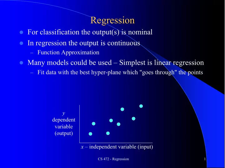
Regression

l For classification the output(s) is nominal l In regression the output is continuous

– Function Approximation

l Many models could be used – Simplest is linear regression

– Fit data with the best hyper-plane which "goes through" the points y dependent variable (output) x – independent variable (input)

CS 472 - Regression 2

Regression

l For classification the output(s) is nominal l In regression the output is continuous

– Function Approximation

l Many models could be used – Simplest is linear regression

– Fit data with the best hyper-plane which "goes through" the points y dependent variable (output) x – independent variable (input)

CS 472 - Regression 3

Regression

l For classification the output(s) is nominal l In regression the output is continuous

– Function Approximation

l Many models could be used – Simplest is linear regression

– Fit data with the best hyper-plane which "goes through" the points – For each point the difference between the predicted point and the

actual observation is the residue

y x

Simple Linear Regression

l For now, assume just one (input) independent variable x,

and one (output) dependent variable y

– Multiple linear regression assumes an input vector x – Multivariate linear regression assumes an output vector y

l We "fit" the points with a line (i.e. hyper-plane) l Which line should we use?

– Choose an objective function – For simple linear regression we choose sum squared error (SSE)

l S (predictedi – actuali)2 =S (residuei)2

– Thus, find the line which minimizes the sum of the squared

residues (e.g. least squares)

– This mimics the case where data points were sampled from the

actual hyperplane with Gaussian noise added

CS 472 - Regression 4

How do we "learn" parameters

l For the 2-d problem (line) there are coefficients for the

bias and the independent variable (y-intercept and slope)

l To find the values for the coefficients which minimize the

• bjective function we take the partial derivates of the
• bjective function (SSE) with respect to the coefficients.

Set these to 0, and solve.

CS 472 - Regression 5

Y = β0 + β1X

β

1 =

n xy

∑

− x y

∑ ∑

n x 2 − x

∑

( )

2

∑

β0 = y

∑

− β

1

x

∑

n

Multiple Linear Regression

l There is a closed form for finding multiple linear regression

weights which requires matrix inversion, etc.

l There are also iterative techniques to find weights l One is the delta rule. For regression we use an output node

which is not thresholded (just does a linear sum) and iteratively apply the delta rule – thus the net is the output

l Where c is the learning rate and x is the input for that weight l Delta rule will update towards the objective of minimizing the

SSE, thus solving multiple linear regression

l There are other regression approaches that give different results

by trying to better handle outliers and other statistical anomalies

CS 472 - Regression 6

Y = β0 + β

1X1 + β2X2 +…+ βnXn

Δwi = c(t − net)xi

SSE and Linear Regression

l SSE chooses to square the difference of

the predicted vs actual. Why square?

l Don't want residues to cancel each other l Could use absolute or other distances to

solve problem

S |predictedi – actuali| : L1 vs L2

l SSE leads to a parabolic error surface

which is good for gradient descent

l Which line would least squares choose?

– There is always one “best” fit

CS 472 - Regression 7

SSE and Linear Regression

l SSE leads to a parabolic error

surface which is good for gradient descent

l Which line would least squares

choose?

– There is always one “best” fit

CS 472 - Regression 8

7

SSE and Linear Regression

l SSE leads to a parabolic error

surface which is good for gradient descent

l Which line would least squares

choose?

– There is always one “best” fit

CS 472 - Regression 9

7 5

SSE and Linear Regression

l SSE leads to a parabolic error

surface which is good for gradient descent

l Which line would least squares

choose?

– There is always one “best” fit

l Note that the squared error causes

the model to be more highly influenced by outliers

– Though best fit assuming Gaussian noise

error from true surface

CS 472 - Regression 10

3 3 7 5

SSE and Linear Regression Generalization

CS 472 - Regression 11

3 3 7 5

l In generalization all x

values map to a y value on the chosen regression line

x – Input Value y – Input Value

1 2 3 1

Linear Regression - Challenge Question

l Assume we start with all weights as 1 (don’t use bias weight though

you usually always will – else forces the line through the origin)

l Remember for regression we use an output node which is not

thresholded (just does a linear sum) and iteratively apply the delta rule – thus the net is the output

l What are the new weights after one iteration through the following

training set using the delta rule with a learning rate c = 1

l How does it generalize for the novel input (-.3, 0)?

CS 472 - Regression 12

x1 x2 Target y .5

• .2

1 1

• .4

Δwi = c(t − net)xi

l After one epoch the weight vector is:

A.

1 .5

B.

1.35 .94

C.

1.35 .86

D.

.4 .86

E.

None of the above

Linear Regression - Challenge Question

l Assume we start with all weights as 1 l What are the new weights after one iteration through the

training set using the delta rule with a learning rate c = 1

l How does it generalize for the novel input (-.3, 0)?

CS 472 - Regression 13

Δwi = c(t − net)xi

x1 x2 Target Net w1 w2 1 1 .5

• .2

1 1

• .4

w1 = 1 +

Linear Regression - Challenge Question

l Assume we start with all weights as 1 l What are the new weights after one iteration through the

training set using the delta rule with a learning rate c = 1

l How does it generalize for the novel input (-.3, 0)?

– -.3*-.4 + 0*.86 = .12

CS 472 - Regression 14

Δwi = c(t − net)xi

x1 x2 Target Net w1 w2 1 1 .5

• .2

1 .3 1.35 .86 1

• .4

1.35

• .4

.86

w1 = 1 + 1(1 – .3).5 = 1.35

Linear Regression Homework

l Assume we start with all weights as 0 (Include the bias!) l What are the new weights after one iteration through the

following training set using the delta rule with a learning rate c = .2

l How does it generalize for the novel input (1, .5)?

CS 472 - Regression 15

x1 x2 Target .3 .8 .7

• .3

1.6

• .1

.9 1.3

Δwi = c(t − net)xi

Intelligibility (Interpretable ML, Transparent)

l One advantage of linear regression models (and linear

classification) is the potential to look at the coefficients to give insight into which input variables are most important in predicting the output

l The variables with the largest magnitude have the highest

correlation with the output

– A large positive coefficient implies that the output will increase when

this input is increased (positively correlated)

– A large negative coefficient implies that the output will decrease when

this input is increased (negatively correlated)

– A small or 0 coefficient suggests that the input is uncorrelated with the

• utput (at least at the 1st order)

l Linear regression can be used to find best "indicators"

– Be careful not to confuse correlation with causality – Linear cannot detect higher order correlations!! The power of more

complex machine learning models.

CS 472 - Regression 16

Anscombe's Quartet

What lines "really" best fit each case? – different approaches

CS 472 - Regression 17

Delta rule natural for regression, not classification

l

First consider the one dimensional case

l

The decision surface for the perceptron would be any (first) point that divides instances

l

Delta rule will try to fit a line through the target values which minimizes SSE and the decision point is where the line crosses .5 for 0/1 targets. Look down

• n data for perceptron view. Now flip it on its side for delta rule view.

l

Will converge to the one optimal line (and dividing point) for this objective

CS 472 - Regression 18

x x z 1

Δwi = c(t − net)xi

Delta Rule for Classification?

l

What would happen in this adjusted case for perceptron and delta rule and where would the decision point (i.e. .5 crossing) be?

CS 472 - Regression 19

x z 1 x z 1

Delta Rule for Classification?

CS 472 - Regression 20

x z 1 x z 1

l

Leads to misclassifications even though the data is linearly separable

l

For Delta rule the objective function is to minimize the regression line SSE, not maximize classification

Delta Rule for Classification?

l

What would happen if we were doing a regression fit with a sigmoid/logistic curve rather than a line?

CS 472 - Regression 21

x z 1 x z 1 x z 1

Delta Rule for Classification?

l

Sigmoid fits many decision cases quite well! This is basically what logistic regression does.

CS 472 - Regression 22

x z 1 x z 1 x z 1

23 1

Observation: Consider the 2 input perceptron case without a bias weight. Note that the output z is a function of 2 input variables for the 2 input case (x1, x2), and thus we really have a 3-d decision surface (i.e. a plane accounting for the two input variables and the 3rd dimension for the output), yet the decision boundary is still a line in the 2- d input space when we represent the outputs with different colors, symbols, etc. The Delta rule would fit a regression plane to these points with the decision line being that line where the plane went through .5. What would logistic regression do?

θ θ < = ≥

∑ ∑

= = i n i i i n i i

w x z w x

1 1

if if 1

CS 472 - Regression

CS 472 - Regression 24

Logistic Regression

l One commonly used algorithm is Logistic Regression l Assumes that the dependent (output) variable is binary

which is often the case in medical and other studies. (Does person have disease or not, survive or not, accepted or not, etc.)

l Like Quadric, Logistic Regression does a particular non-

linear transform on the data after which it just does linear regression on the transformed data

l Logistic regression fits the data with a sigmoidal/logistic

curve rather than a line and outputs an approximation of the probability of the output given the input

CS 472 - Regression 25

Logistic Regression Example

l Age (X axis, input variable) – Data is fictional l Heart Failure (Y axis, 1 or 0, output variable) l If use value of regression line as a probability approximation

–

Extrapolates outside 0-1 and not as good empirically

l Sigmoidal curve to the right gives empirically good probability

approximation and is bounded between 0 and 1

CS 472 - Regression 26

Logistic Regression Approach

Learning

1.

Transform initial input probabilities into log odds (logit)

2.

Do a standard linear regression on the logit values

–

This effectively fits a logistic curve to the data, while still just doing a linear regression with the transformed input (ala quadric machine, etc.)

Generalization

1.

Find the value for the new input on the logit line

2.

Transform that logit value back into a probability

CS 472 - Regression 27

Non-Linear Pre-Process to Logit (Log Odds)

CS 472 - Regression 28

Medication Dosage # Cured Total Patients Probability: # Cured/Total Patients 20 1 5 .20 30 2 6 .33 40 4 6 .67 50 6 7 .86 0 10 20 30 40 50 60 Cured Not Cured 0 10 20 30 40 50 60 prob. Cured 1

Non-Linear Pre-Process to Logit (Log Odds)

CS 472 - Regression 29

Medication Dosage # Cured Total Patients Probability: # Cured/Total Patients 20 1 5 .20 30 2 6 .33 40 4 6 .67 50 6 7 .86 0 10 20 30 40 50 60 Cured Not Cured 0 10 20 30 40 50 60 prob. Cured 1

Logistic Regression Approach

l Could use linear regression with the probability points, but

that would not extrapolate well

l Logistic version is better but how do we get it? l Similar to Quadric we do a non-linear pre-process of the

input and then do linear regression on the transformed values – do a linear regression on the log odds - Logit

CS 472 - Regression 30

0 10 20 30 40 50 60 prob. Cured 1 0 10 20 30 40 50 60 prob. Cured 1

Non-Linear Pre-Process to Logit (Log Odds)

CS 472 - Regression 31

Medication Dosage # Cured Total Patients Probability: # Cured/Total Patients Odds: p/(1-p) = # cured/ # not cured Logit Log Odds: ln(Odds) 20 1 5 .20 .25

• 1.39

30 2 6 .33 .50

• 0.69

40 4 6 .67 2.0 0.69 50 6 7 .86 6.0 1.79 0 10 20 30 40 50 60 Cured Not Cured 0 10 20 30 40 50 60 prob. Cured 1

Regression of Log Odds

CS 472 - Regression 32

Medication Dosage # Cured Total Patients Probability: # Cured/Total Patients Odds: p/(1-p) = # cured/ # not cured Log Odds: ln(Odds)

20 1 5 .20 .25

• 1.39

30 2 6 .33 .50

• 0.69

40 4 6 .67 2.0 0.69 50 6 7 .86 6.0 1.79 0 10 20 30 40 50 60 +2

• 2
• y = .11x – 3.8 - Logit regression equation
• Now we have a regression line for log odds (logit)
• To generalize, we use the log odds value for the new data point
• Then we transform that log odds point to a probability: p = elogit(x)/(1+elogit(x))
• For example assume we want p for dosage = 10

Logit(10) = .11(10) – 3.8 = -2.7 p(10) = e-2.7/(1+e-2.7) = .06 [note that we just work backwards from logit to p]

• These p values make up the sigmoidal regression curve (which we never have to

actually plot)

prob. Cured

1

Logistic Regression Homework

l You don’t actually have to come up with the weights for this one,

though you could do so quickly by using the closed form linear regression approach

l Sketch each step you would need to learn the weights for the following

data set using logistic regression

l Sketch how you would generalize the probability of a heart attack

given a new input heart rate of 60

CS 472 - Regression 33

Heart Rate Heart Attack 50 Y 50 N 50 N 50 N 70 N 70 Y 90 Y 90 Y 90 N 90 Y 90 Y

Summary

l Linear Regression and Logistic Regression are nice tools

for many simple situations

– But both force us to fit the data with one shape (line or sigmoid)

which will often underfit

l Intelligible results l When problem includes more arbitrary non-linearity then

we need more powerful models which we will introduce

– Though non-linear data transformation can help in these cases

while still using a linear model for learning

l These models are commonly used in data mining

applications and also as a "first attempt" at understanding data trends, indicators, etc.

CS 472 - Regression 34

Non-Linear Regression

l All of the classification models which we will be

discussing later in class can also be used for non-linear regression

– MLP with Backpropagation, Decision Trees, Nearest Neighbor,

etc.

l They can learn to learn functions with arbitrarily complex

high dimensional surfaces

CS 472 - Regression 35