CSCE 478/878 Lecture 6: Bayesian Learning MAP learners 1. Provide - PowerPoint PPT Presentation

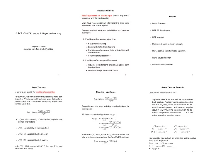
Bayesian Methods Not all hypotheses are created equal (even if they are all Outline consistent with the training data) Might have reasons (domain information) to favor some • Bayes Theorem hypotheses over others a priori Bayesian methods work with probabilities, and have two • MAP , ML hypotheses main roles: CSCE 478/878 Lecture 6: Bayesian Learning • MAP learners 1. Provide practical learning algorithms: • Na¨ ıve Bayes learning • Minimum description length principle Stephen D. Scott • Bayesian belief network learning (Adapted from Tom Mitchell’s slides) • Combine prior knowledge (prior probabilities) with • Bayes optimal classifier/Gibbs algorithm observed data • Requires prior probabilities • Na¨ ıve Bayes classifier 2. Provides useful conceptual framework • Bayesian belief networks • Provides “gold standard” for evaluating other learn- ing algorithms • Additional insight into Occam’s razor 1 2 3 Bayes Theorem Bayes Theorem Example In general, an identity for conditional probabilities Choosing Hypotheses Does patient have cancer or not? For our work, we want to know the probability that a par- P ( h | D ) = P ( D | h ) P ( h ) ticular h ∈ H is the correct hypothesis given that we have A patient takes a lab test and the result comes P ( D ) seen training data D (examples and labels). Bayes theo- back positive. The test returns a correct positive rem lets us do this. result in only 98% of the cases in which the dis- Generally want the most probable hypothesis given the ease is actually present, and a correct negative training data result in only 97% of the cases in which the dis- P ( h | D ) = P ( D | h ) P ( h ) ease is not present. Furthermore, 0 . 008 of the P ( D ) Maximum a posteriori hypothesis h MAP : entire population have this cancer. h MAP = argmax P ( h | D ) • P ( h ) = prior probability of hypothesis h (might include h ∈ H domain information) P ( D | h ) P ( h ) = argmax P ( D ) h ∈ H P ( cancer ) = P ( ¬ cancer ) = = argmax P ( D | h ) P ( h ) • P ( D ) = probability of training data D P (+ | cancer ) = P ( − | cancer ) = h ∈ H P (+ | ¬ cancer ) = P ( − |¬ cancer ) = • P ( h | D ) = probability of h given D If assume P ( h i ) = P ( h j ) for all i, j , then can further sim- plify, and choose the maximum likelihood (ML) hypothesis Now consider new patient for whom the test is positive. • P ( D | h ) = probability of D given h What is our diagnosis? h ML = argmax P ( D | h i ) h i ∈ H P (+ | cancer ) P ( cancer ) = P (+ | ¬ cancer ) P ( ¬ cancer ) = Note P ( h | D ) increases with P ( D | h ) and P ( h ) and decreases with P ( D ) So h MAP = 4 5 6

Basic Formulas for Probabilities Brute Force MAP Hypothesis Learner • Product Rule : probability P ( A ∧ B ) of a conjunction Relation to Concept Learning of two events A and B: 1. For each hypothesis h in H , calculate the posterior Consider our usual concept learning task: instance space P ( A ∧ B ) = P ( A | B ) P ( B ) = P ( B | A ) P ( A ) probability X , hypothesis space H , training examples D P ( h | D ) = P ( D | h ) P ( h ) P ( D ) • Sum Rule : probability of a disjunction of two events A Consider the Find-S learning algorithm (outputs most spe- and B: cific hypothesis from the version space V S H,D ) 2. Output the hypothesis h MAP with the highest poste- P ( A ∨ B ) = P ( A ) + P ( B ) − P ( A ∧ B ) rior probability What would brute-force MAP learner output as MAP hy- pothesis? h MAP = argmax P ( h | D ) • Theorem of total probability : if events A 1 , . . . , A n are h ∈ H mutually exclusive with � n i =1 P ( A i ) = 1 , then Does Find-S output a MAP hypothesis?? n Problem: what if H exponentially or infinitely large? � P ( B ) = P ( B | A i ) P ( A i ) i =1 7 8 9 Relation to Concept Learning Characterizing Learning Algorithms by Equivalent (cont’d) MAP Learners Inductive system Learning A Real-Valued Function Assume fixed set of instances � x 1 , . . . , x m � Training examples D Output hypotheses Candidate Elimination Consider any real-valued target function f Hypothesis space H Algorithm Assume D is the set of classifications D = � c ( x 1 ) , . . . , c ( x m ) � Training examples � x i , d i � , where d i is noisy training value Equivalent Bayesian inference system Assume no noise and c ∈ H , so choose  Training examples D 1 if d i = h ( x i ) for all d i ∈ D   • d i = f ( x i ) + e i Output hypotheses P ( D | h ) = Hypothesis space H   0 otherwise Brute force MAP learner • e i is random variable (noise) drawn independently for P(h) uniform P(D|h) = 0 if inconsistent, each x i according to some Gaussian distribution with = 1 if consistent Choose P ( h ) = 1 / | H | ∀ h ∈ H , i.e. uniform dist. mean µ e i = 0 If h inconsistent with D , then Prior assumptions made explicit P ( h | D ) = (0 · P ( h )) /P ( D ) = 0 Then the maximum likelihood hypothesis h ML is the one that minimizes the sum of squared errors, e.g. a linear unit So we can characterize algorithms in a Bayesian frame- trained with GD/EG: If h consistent with D , then � � work even though they don’t directly manipulate probabili- m P ( h | D ) = (1 · 1 / | H | ) /P ( D ) = (1 / | H | ) / | V S H,D | / | H | � ( d i − h ( x i )) 2 ties h ML = argmin = 1 / | V S H,D | (see Thrm of total prob., slide 7) h ∈ H i =1 Other priors will allow Find-S, etc. to output MAP; e.g. Thus if D noise-free and c ∈ H and P ( h ) uniform, P ( h ) that favors more specific hypotheses every consistent hypothesis is a MAP hypothesis 10 11 12

Learning A Real-Valued Function (cont’d) Learning to Predict Probabilities Minimum Description Length Principle h ML = argmax p ( D | h ) = argmax p ( d 1 , . . . , d m | h ) h ∈ H h ∈ H Consider predicting survival probability from patient data m Occam’s razor: prefer the shortest hypothesis � = argmax p ( d i | h ) (if d i ’s cond. indep.) h ∈ H i =1 Training examples � x i , d i � , where d i is 1 or 0  � 2  � MDL: prefer the hypothesis h that satisfies m 1  − 1 d i − h ( x i ) (assume label is [or appears] probabilistically generated) � √ = argmax 2 πσ 2 exp  2 h ∈ H σ h MDL = argmin L C 1 ( h ) + L C 2 ( D | h ) i =1 h ∈ H Want to train neural network to output the probability that ( µ e i = 0 ⇒ E [ d i | h ] = h ( x i ) ) where L C ( x ) is the description length of x under encoding x i has label 1, not the label itself C Maximize natural log instead: Using approach similar to previous slide (p. 169), can show � 2 m � 2 πσ 2 − 1 1 d i − h ( x i ) � Example: H = decision trees, D = training data labels h ML = argmax ln √ m 2 � h ∈ H σ h ML = argmax d i ln h ( x i )+(1 − d i ) ln(1 − h ( x i )) i =1 • L C 1 ( h ) is # bits to describe tree h � 2 h ∈ H m � i =1 − 1 d i − h ( x i ) � = argmax i.e. find h minimizing cross-entropy • L C 2 ( D | h ) is # bits to describe D given h 2 h ∈ H σ i =1 m � − ( d i − h ( x i )) 2 = argmax – Note L C 2 ( D | h ) = 0 if examples classified per- For single sigmoid unit, use update rule h ∈ H i =1 fectly by h (need only describe exceptions) m m � � ( d i − h ( x i )) 2 w j ← w j + η ( d i − h ( x i )) x ij = argmin • Hence h MDL trades off tree size for training errors h ∈ H i =1 i =1 to find h ML (can also derive EG rule) Thus have Bayesian justification for minimizing squared error (under certain assumptions) 13 14 15 Minimum Description Length Principle Bayes Optimal Classifier Bayesian Justification (cont’d) Bayes Optimal Classifier Bayes optimal classification: h MAP = argmax P ( D | h ) P ( h ) h ∈ H � • So far we’ve sought the most probable hypothesis given argmax P ( v j | h i ) P ( h i | D ) = argmax log 2 P ( D | h ) + log 2 P ( h ) v j ∈ V the data D , i.e. h MAP h i ∈ H h ∈ H = argmin − log 2 P ( D | h ) − log 2 P ( h ) (1) where V is set of possible labels (e.g. { + , − } ) h ∈ H • But given new instance x , h MAP ( x ) is not necessar- Example: Interesting fact from information theory: The optimal (short- ily the most probable classification! est expected coding length) code for an event with proba- P ( h 1 | D ) = 0 . 4 , P ( − | h 1 ) = 0 , P (+ | h 1 ) = 1 bility p is − log 2 p bits. P ( h 2 | D ) = 0 . 3 , P ( − | h 2 ) = 1 , P (+ | h 2 ) = 0 • Consider three possible hypotheses: P ( h 3 | D ) = 0 . 3 , P ( − | h 3 ) = 1 , P (+ | h 3 ) = 0 So interpret (1): therefore P ( h 1 | D ) = 0 . 4 , P ( h 2 | D ) = 0 . 3 , P ( h 3 | D ) = 0 . 3 • − log 2 P ( h ) is length of h under optimal code � P (+ | h i ) P ( h i | D ) = 0 . 4 Given new instance x , h i ∈ H • − log 2 P ( D | h ) is length of D given h under optimal h 1 ( x ) = + , h 2 ( x ) = − , h 3 ( x ) = − � P ( − | h i ) P ( h i | D ) = 0 . 6 code h i ∈ H → prefer the hypothesis that minimizes and • h MAP ( x ) = � length ( h ) + length ( misclassifications ) argmax P ( v j | h i ) P ( h i | D ) = − v j ∈ V h i ∈ H • What’s the most probable classification of x ? Caveat: h MDL = h MAP doesn’t apply for arbitrary en- On average, no other classifier using same prior and codings (need P ( h ) and P ( D | h ) to be optimal); merely same hyp. space can outperform Bayes optimal! a guide 16 17 18