Probability Intro Part II: Bayes Rule Jonathan Pillow Mathematical - PowerPoint PPT Presentation
Probability Intro Part II: Bayes Rule Jonathan Pillow Mathematical Tools for Neuroscience (NEU 314) Spring, 2016 lecture 13 Quick recap Random variable X takes on different values according to a probability distribution discrete:
Probability Intro Part II: Bayes’ Rule Jonathan Pillow Mathematical Tools for Neuroscience (NEU 314) Spring, 2016 lecture 13
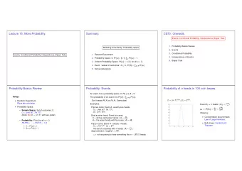
Quick recap • Random variable X takes on different values according to a probability distribution • discrete: probability mass function (pmf) • continuous: probability density function (pdf) • marginalization : summing (“splatting”) • conditionalization: “slicing”
conditionalization (“slicing”) 3 2 (“joint divided by marginal”) 1 0 − 1 − 2 − 3 -3 -2 -1 0 1 2 3 − 3 − 2 − 1 0 1 2 3
conditionalization (“slicing”) 3 2 (“joint divided by marginal”) 1 0 − 1 − 2 − 3 -3 -2 -1 0 1 2 3 − 3 − 2 − 1 0 1 2 3
conditionalization (“slicing”) conditional 3 2 1 0 marginal − 1 P(x) − 2 − 3 -3 -2 -1 0 1 2 3 − 3 − 2 − 1 0 1 2 3
conditional densities 3 2 1 0 − 1 − 2 − 3 -3 -2 -1 0 1 2 3 − 3 − 2 − 1 0 1 2 3
conditional densities 3 2 1 0 − 1 − 2 − 3 -3 -2 -1 0 1 2 3 − 3 − 2 − 1 0 1 2 3
Bayes’ Rule Conditional Densities likelihood prior Bayes’ Rule marginal probability of y posterior (“normalizer”)
A little math: Bayes’ rule • very simple formula for manipulating probabilities P(A | B) P(B) P(B | A) = probability of B P(A) conditional probability probability of A “probability of B given that A occurred” P(B | A) ∝ P(A | B) P(B) simplified form:
A little math: Bayes’ rule P(B | A) ∝ P(A | B) P(B) Example: 2 coins • one coin is fake: “heads” on both sides (H / H) • one coin is standard: (H / T) You grab one of the coins at random and flip it. It comes up “heads”. What is the probability that you’re holding the fake? ∝ p(H | Fake) p(Fake) p( Fake | H) ( 1 ) ( ½ ) = ½ ∝ p (H | Nrml) p(Nrml) p( Nrml | H) ( ½ ) ( ½ ) = ¼ probabilities must sum to 1
A little math: Bayes’ rule P(B | A) ∝ P(A | B) P(B) start Example: 2 coins fake normal H T H H ∝ p(H | Fake) p(Fake) p( Fake | H) ( 1 ) ( ½ ) = ½ ∝ p (H | Nrml) p(Nrml) p( Nrml | H) ( ½ ) ( ½ ) = ¼ probabilities must sum to 1
A little math: Bayes’ rule P(B | A) ∝ P(A | B) P(B) start Example: 2 coins fake normal H T H H Experiment #2: It comes up “tails”. What is the probability that you’re holding the fake? ∝ p(T | Fake) p(Fake) p( Fake | T) ( 0 ) ( ½ ) = 0 = 0 ∝ p (T | Nrml) p(Nrml) p( Nrml | T) probabilities must sum to 1 ( ½ ) ( ½ ) = ¼ = 1
Is the middle circle popping “out” or “in”?
P( image | OUT & light is above) = 1 P(image | IN & Light is below) = 1 • Image equally likely to be OUT or IN given sensory data alone What we want to know: P(OUT | image) vs. P(IN | image) Apply Bayes’ rule: prior P(OUT | image) ∝ P(image | OUT & light above) × P(OUT) × P(light above) P(IN | image) ∝ P(image | IN & light below ) × P(IN) × P(light below) Which of these is greater?
Bayesian Models for Perception P(B | A) ∝ P(A | B) P(B) Bayes’ rule: P(what’s in the world | sensory data) Formula for computing: (This is what our brain wants to know!) B A P(world | sense data) ∝ P(sense data | world) P(world) Likelihood Prior Posterior (given by past experience) (given by laws of physics; (resulting beliefs about ambiguous because many world states the world) could give rise to same sense data)
Helmholtz: perception as “optimal inference” “Perception is our best guess as to what is in the world, given our current sensory evidence and our prior experience.” helmholtz 1821-1894 P(world | sense data) ∝ P(sense data | world) P(world) Likelihood Prior Posterior (given by past experience) (given by laws of physics; (resulting beliefs about ambiguous because many world states the world) could give rise to same sense data)
Helmholtz: perception as “optimal inference” “Perception is our best guess as to what is in the world, given our current sensory evidence and our prior experience .” helmholtz 1821-1894 P(world | sense data) ∝ P(sense data | world) P(world) Likelihood Prior Posterior (given by past experience) (given by laws of physics; (resulting beliefs about ambiguous because many world states the world) could give rise to same sense data)
Many different 3D scenes can give rise to the same 2D retinal image The Ames Room
Many different 3D scenes can give rise to the same 2D retinal image The Ames Room A B How does our brain go about deciding which interpretation? P(image | A) and P(image | B) are equal! (both A and B could have generated this image) Let’s use Bayes’ rule: P(A | image) = P(image | A) P(A) / Z P(B | image) = P(image | B) P(B) / Z
Hollow Face Illusion http://www.richardgregory.org/experiments/
∴ Hollow Face Illusion ex ve eo Hypothesis #1: face is concave Hypothesis #2: face is convex P(convex|video) ∝ P(video|convex) P(convex) P(concave|video) ∝ P(video|concave) P(concave) posterior likelihood prior P(convex) > P(concave) ⇒ posterior probability of convex is higher (which determines our percept)
• prior belief that objects are convex is SO strong we can’t over-ride it, even when we know it’s wrong! (So your brain knows Bayes’ rule even if you don’t!)
Terminology question: • When do we call this a likelihood ? A : when considered as a function of x (i.e., with y held fixed) • note: doesn’t integrate to 1 . • What’s it called as a function of y, for fixed x? conditional distribution or sampling distribution
independence 3 2 1 0 − 1 − 2 − 3 − 3 − 2 − 1 0 1 2 3
independence Definition: x , y are independent iff 3 2 1 0 − 1 − 2 − 3 − 3 − 2 − 1 0 1 2 3
independence Definition: x , y are independent iff 3 2 In linear algebra terms: 1 0 (outer product) − 1 − 2 − 3 − 3 − 2 − 1 0 1 2 3
Summary • marginalization (splatting) • conditionalization (slicing) • Bayes’ rule (prior, likelihood, posterior) • independence
Recommend
More recommend
Explore More Topics
Stay informed with curated content and fresh updates.
