CSCE 478/878 Lecture 5: Evaluating will misclassify an instance - PowerPoint PPT Presentation

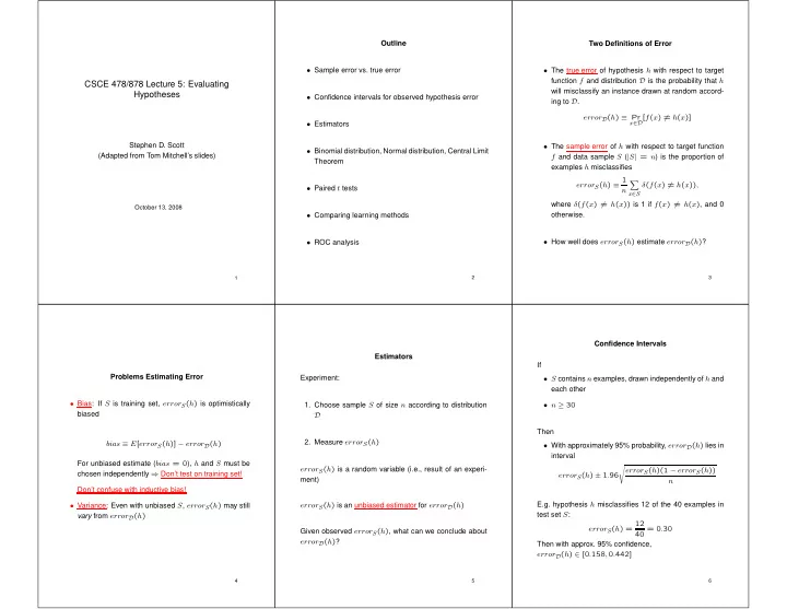
Outline Two Definitions of Error • Sample error vs. true error • The true error of hypothesis h with respect to target function f and distribution D is the probability that h CSCE 478/878 Lecture 5: Evaluating will misclassify an instance drawn at random accord- Hypotheses • Confidence intervals for observed hypothesis error ing to D . error D ( h ) ≡ Pr x ∈D [ f ( x ) � = h ( x )] • Estimators Stephen D. Scott • The sample error of h with respect to target function • Binomial distribution, Normal distribution, Central Limit (Adapted from Tom Mitchell’s slides) f and data sample S ( | S | = n ) is the proportion of Theorem examples h misclassifies error S ( h ) ≡ 1 � δ ( f ( x ) � = h ( x )) , • Paired t tests n x ∈ S where δ ( f ( x ) � = h ( x )) is 1 if f ( x ) � = h ( x ) , and 0 October 13 , 200 8 otherwise. • Comparing learning methods • How well does error S ( h ) estimate error D ( h ) ? • ROC analysis 2 3 1 Confidence Intervals Estimators If Problems Estimating Error Experiment: • S contains n examples, drawn independently of h and each other • Bias: If S is training set, error S ( h ) is optimistically 1. Choose sample S of size n according to distribution • n ≥ 30 biased D Then 2. Measure error S ( h ) bias ≡ E [ error S ( h )] − error D ( h ) • With approximately 95% probability, error D ( h ) lies in interval For unbiased estimate ( bias = 0 ), h and S must be � error S ( h ) is a random variable (i.e., result of an experi- error S ( h )(1 − error S ( h )) chosen independently ⇒ Don’t test on training set! error S ( h ) ± 1 . 96 ment) n Don’t confuse with inductive bias! E.g. hypothesis h misclassifies 12 of the 40 examples in • Variance: Even with unbiased S , error S ( h ) may still error S ( h ) is an unbiased estimator for error D ( h ) test set S : vary from error D ( h ) error S ( h ) = 12 40 = 0 . 30 Given observed error S ( h ) , what can we conclude about error D ( h ) ? Then with approx. 95% confidence, error D ( h ) ∈ [0 . 158 , 0 . 442] 4 5 6

Binomial Probability Distribution Binomial distribution for n = 40, p = 0.3 0.14 error S ( h ) is a Random Variable 0.12 Confidence Intervals 0.1 (cont’d) 0.08 P(r) Repeatedly run the experiment, each with different ran- 0.06 domly drawn S (each of size n ) 0.04 If 0.02 0 0 5 10 15 20 25 30 35 40 • S contains n examples, drawn independently of h and Probability of observing r misclassified examples: each other Binomial distribution for n = 40, p = 0.3 0.14 � n n ! p r (1 − p ) n − r = � r !( n − r )! p r (1 − p ) n − r P ( r ) = 0.12 • n ≥ 30 r 0.1 P(r) 0.08 0.06 Probability P ( r ) of r heads in n coin flips, if p = Pr( heads ) 0.04 Then 0.02 • Expected, or mean value of X , E [ X ] (= # heads on n 0 • With approximately N % probability, error D ( h ) lies in 0 5 10 15 20 25 30 35 40 flips = # mistakes on n test exs), is interval n � � E [ X ] ≡ iP ( i ) = np = n · error D ( h ) error S ( h )(1 − error S ( h )) error S ( h ) ± z N � n i =0 error D ( h ) r (1 − error D ( h )) n − r � n P ( r ) = r where • Variance of X is N % : 50% 68% 80% 90% 95% 98% 99% I.e. let error D ( h ) be probability of heads in biased coin, V ar ( X ) ≡ E [( X − E [ X ]) 2 ] = np (1 − p ) z N : 0.67 1.00 1.28 1.64 1.96 2.33 2.58 the P ( r ) = prob. of getting r heads out of n flips Why? • Standard deviation of X , σ X , is What kind of distribution is this? � E [( X − E [ X ]) 2 ] = � σ X ≡ np (1 − p ) 7 8 9 Normal Probability Distribution Normal Probability Distribution Normal distribution with mean 0, standard deviation 1 Approximate Binomial Dist. with Normal (cont’d) 0.4 0.35 0.3 0.25 0.4 error S ( h ) = r/n is binomially distributed, with 0.2 0.35 0.15 0.3 0.1 0.25 • mean µ error S ( h ) = error D ( h ) (i.e. unbiased est.) 0.05 0.2 0 0.15 -3 -2 -1 0 1 2 3 0.1 • standard deviation σ error S ( h ) 0.05 0 -3 -2 -1 0 1 2 3 � error D ( h )(1 − error D ( h )) � 2 � 1 � − 1 � x − µ 80% of area (probability) lies in µ ± 1 . 28 σ σ error S ( h ) = p ( x ) = √ 2 πσ 2 exp n 2 σ N % of area (probability) lies in µ ± z N σ (i.e. increasing n decreases variance) N % : 50% 68% 80% 90% 95% 98% 99% • Defined completely by µ and σ z N : 0.67 1.00 1.28 1.64 1.96 2.33 2.58 Want to compute confidence interval = interval centered • The probability that X will fall into the interval ( a, b ) is at error D ( h ) containing N % of the weight under the dis- given by Can also have one-sided bounds: � b tribution (difficult for binomial) 0.4 0.35 a p ( x ) dx 0.3 0.25 Approximate binomial by normal (Gaussian) dist: 0.2 0.15 • Expected, or mean value of X , E [ X ] , is 0.1 • mean µ error S ( h ) = error D ( h ) 0.05 E [ X ] = µ 0 -3 -2 -1 0 1 2 3 • standard deviation σ error S ( h ) • Variance of X is V ar ( X ) = σ 2 N % of area lies < µ + z ′ N σ or > µ − z ′ N σ , where z ′ N = � error S ( h )(1 − error S ( h )) z 100 − (100 − N ) / 2 σ error S ( h ) ≈ • Standard deviation of X , σ X , is n N % : 50% 68% 80% 90% 95% 98% 99% σ X = σ z ′ N : 0.0 0.47 0.84 1.28 1.64 2.05 2.33 10 11 12

Confidence Intervals Revisited Central Limit Theorem Calculating Confidence Intervals If How can we justify approximation? 1. Pick parameter p to estimate • S contains n examples, drawn independently of h and each other Consider a set of independent, identically distributed ran- • error D ( h ) dom variables Y 1 . . . Y n , all governed by an arbitrary prob- • n ≥ 30 ability distribution with mean µ and finite variance σ 2 . De- fine the sample mean 2. Choose an estimator Then n • With approximately 95% probability, error S ( h ) lies in Y ≡ 1 ¯ • error S ( h ) � Y i interval n i =1 � error D ( h )(1 − error D ( h )) error D ( h ) ± 1 . 96 3. Determine probability distribution that governs esti- n Note that ¯ Y is itself a random variable, i.e. the result of an mator experiment (e.g. error S ( h ) = r/n ) Equivalently, error D ( h ) lies in interval • error S ( h ) governed by binomial distribution, ap- Central Limit Theorem: As n → ∞ , the distribution gov- � proximated by normal when n ≥ 30 error D ( h )(1 − error D ( h )) error S ( h ) ± 1 . 96 erning ¯ Y approaches a Normal distribution, with mean µ n and variance σ 2 /n 4. Find interval ( L, U ) such that N % of probability mass which is approximately falls in the interval Thus the distribution of error S ( h ) is approximately nor- � error S ( h )(1 − error S ( h )) mal for large n , and its expected value is error D ( h ) error S ( h ) ± 1 . 96 • Could have L = −∞ or U = ∞ n (Rule of thumb: n ≥ 30 when estimator’s distribution is • Use table of z N or z ′ N values (if distrib. normal) (One-sided bounds yield upper or lower error bounds) binomial, might need to be larger for other distributions) 13 14 15 Difference Between Hypotheses Paired t test to compare h A , h B Comparing Learning Algorithms L A and L B Test h 1 on sample S 1 , test h 2 on S 2 , S 1 ∩ S 2 = ∅ 1. Partition data into k disjoint test sets T 1 , T 2 , . . . , T k of equal size, where this size is at least 30 What we’d like to estimate: 1. Pick parameter to estimate 2. For i from 1 to k , do E S ⊂D [ error D ( L A ( S )) − error D ( L B ( S ))] d ≡ error D ( h 1 ) − error D ( h 2 ) where L ( S ) is the hypothesis output by learner L using δ i ← error T i ( h A ) − error T i ( h B ) training set S 2. Choose an estimator 3. Return the value ¯ δ , where ˆ d ≡ error S 1 ( h 1 ) − error S 2 ( h 2 ) I.e., the expected difference in true error between hypothe- k δ ≡ 1 ¯ � δ i (unbiased) ses output by learners L A and L B , when trained using k i =1 randomly selected training sets S drawn according to dis- 3. Determine probability distribution that governs esti- tribution D mator (difference between two normals is also nor- N % confidence interval estimate for d : mal, variances add) But, given limited data D 0 , what is a good estimator? ¯ δ ± t N,k − 1 s ¯ � δ error S 1 ( h 1 )(1 − error S 1 ( h 1 )) + error S 2 ( h 2 )(1 − error S 2 ( h 2 )) σ ˆ d ≈ • Could partition D 0 into training set S 0 and testing set n 1 n 2 � � k 1 T 0 , and measure � 2 � � � δ i − ¯ s ¯ δ ≡ δ � � k ( k − 1) i =1 error T 0 ( L A ( S 0 )) − error T 0 ( L B ( S 0 )) 4. Find interval ( L, U ) such that N % of prob. mass falls in the interval: ˆ d ± z n σ ˆ • Even better, repeat this many times and average the d t plays role of z , s plays role of σ results (next slide) t test gives more accurate results since std. deviation ap- Can also use S = S 1 ∪ S 2 to test h 1 and h 2 proximated and test sets for h A and h B not independent 16 17 18