CSCE 478/878 Lecture 8: Stephen Scott Clustering Introduction - PowerPoint PPT Presentation

CSCE 478/878 Lecture 8: Clustering CSCE 478/878 Lecture 8: Stephen Scott Clustering Introduction Outline Clustering Stephen Scott k -Means Clustering Hierarchical Clustering sscott@cse.unl.edu 1 / 19

Introduction CSCE 478/878 If no label information is available, can still perform Lecture 8: unsupervised learning Clustering Stephen Scott Looking for structural information about instance space instead of label prediction function Introduction Outline Approaches: density estimation, clustering, Clustering dimensionality reduction k -Means Clustering Clustering algorithms group similar instances together Hierarchical based on a similarity measure Clustering x1 x1 Clustering Algorithm x2 x2 2 / 19

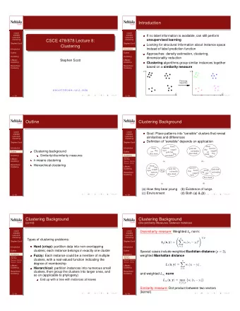
Outline CSCE 478/878 Lecture 8: Clustering Stephen Scott Introduction Clustering background Outline Similarity/dissimilarity measures Clustering k -Means k -means clustering Clustering Hierarchical clustering Hierarchical Clustering 3 / 19

Clustering Background CSCE Goal: Place patterns into “sensible” clusters that reveal 478/878 Lecture 8: similarities and differences Clustering Definition of “sensible” depends on application Stephen Scott Introduction Outline Clustering Measures: Point-Point Measures: Point-Set Measures: Set-Set k -Means Clustering Hierarchical Clustering (a) How they bear young (b) Existence of lungs (c) Environment (d) Both (a) & (b) 4 / 19

Clustering Background (cont’d) CSCE 478/878 Lecture 8: Clustering Types of clustering problems: Stephen Scott Hard (crisp): partition data into non-overlapping Introduction clusters; each instance belongs in exactly one cluster Outline Clustering Fuzzy: Each instance could be a member of multiple Measures: Point-Point clusters, with a real-valued function indicating the Measures: Point-Set Measures: Set-Set degree of membership k -Means Hierarchical: partition instances into numerous small Clustering clusters, then group the clusters into larger ones, and Hierarchical Clustering so on (applicable to phylogeny) End up with a tree with instances at leaves 5 / 19

Clustering Background (Dis-)similarity Measures: Between Instances CSCE Dissimilarity measure: Weighted L p norm: 478/878 Lecture 8: � n Clustering � 1 / p � w i | x i − y i | p Stephen Scott L p ( x , y ) = i = 1 Introduction Outline Special cases include weighted Euclidian distance ( p = 2 ), Clustering weighted Manhattan distance Measures: Point-Point n Measures: Point-Set Measures: Set-Set � L 1 ( x , y ) = w i | x i − y i | , k -Means Clustering i = 1 Hierarchical and weighted L ∞ norm Clustering L ∞ ( x , y ) = max 1 ≤ i ≤ n { w i | x i − y i |} Similarity measure: Dot product between two vectors (kernel) 6 / 19

Clustering Background (Dis-)similarity Measures: Between Instances (cont’d) CSCE 478/878 Lecture 8: Clustering If attributes come from { 0 , . . . , k − 1 } , can use measures for Stephen Scott real-valued attributes, plus: Introduction Outline Hamming distance : DM measuring number of places Clustering where x and y differ Measures: Point-Point Tanimoto measure : SM measuring number of places Measures: Point-Set Measures: Set-Set where x and y are same, divided by total number of k -Means places Clustering Ignore places i where x i = y i = 0 Hierarchical Clustering Useful for ordinal features where x i is degree to which x possesses i th feature 7 / 19

Clustering Background (Dis-)similarity Measures: Between Instance and Set CSCE 478/878 Might want to measure proximity of point x to existing Lecture 8: Clustering cluster C Stephen Scott Can measure proximity α by using all points of C or by Introduction using a representative of C Outline If all points of C used, common choices: Clustering Measures: Point-Point α ps max ( x , C ) = max y ∈ C { α ( x , y ) } Measures: Point-Set Measures: Set-Set k -Means α ps min ( x , C ) = min y ∈ C { α ( x , y ) } Clustering Hierarchical Clustering avg ( x , C ) = 1 α ps � α ( x , y ) , | C | y ∈ C where α ( x , y ) is any measure between x and y 8 / 19

Clustering Background (Dis-)similarity Measures: Between Instance and Set (cont’d) CSCE Alternative: Measure distance between point x and a 478/878 representative of the cluster C Lecture 8: Clustering Mean vector m p = 1 Stephen Scott � y | C | Introduction y ∈ C Mean center m c ∈ C : Outline Clustering � � d ( m c , y ) ≤ d ( z , y ) ∀ z ∈ C , Measures: Point-Point y ∈ C y ∈ C Measures: Point-Set Measures: Set-Set where d ( · , · ) is DM (if SM used, reverse ineq.) k -Means Clustering Median center : For each point y ∈ C , find median Hierarchical dissimilarity from y to all other points of C , then take Clustering min; so m med ∈ C is defined as med y ∈ C { d ( m med , y ) } ≤ med y ∈ C { d ( z , y ) } ∀ z ∈ C Now can measure proximity between C ’s representative and x with standard measures 9 / 19

Clustering Background (Dis-)similarity Measures: Between Sets CSCE 478/878 Lecture 8: Clustering Given sets of instances C i and C j and proximity measure Stephen Scott α ( · , · ) Introduction Outline Max : α ss max ( C i , C j ) = x ∈ C i , y ∈ C j { α ( x , y ) } max Clustering Measures: Min : α ss min ( C i , C j ) = x ∈ C i , y ∈ C j { α ( x , y ) } Point-Point min Measures: Point-Set Measures: Set-Set 1 k -Means � � Average : α ss avg ( C i , C j ) = α ( x , y ) Clustering | C i | | C j | Hierarchical x ∈ C i y ∈ C j Clustering Representative (mean) : α ss mean ( C i , C j ) = α ( m C i , m C j ) , 10 / 19

k -Means Clustering CSCE 478/878 Lecture 8: Very popular clustering algorithm Clustering Represents cluster i (out of k total) by specifying its Stephen Scott representative m i (not necessarily part of the original Introduction set of instances X ) Outline Each instance x ∈ X is assigned to the cluster with Clustering nearest representative k -Means Clustering Goal is to find a set of k representatives such that sum Algorithm Example of distances between instances and their Hierarchical representatives is minimized Clustering NP-hard in general Will use an algorithm that alternates between determining representatives and assigning clusters until convergence (in the style of the EM algorithm) 11 / 19

k -Means Clustering Algorithm CSCE 478/878 Lecture 8: Clustering Choose value for parameter k Stephen Scott Initialize k arbitrary representatives m 1 , . . . , m k Introduction E.g., k randomly selected instances from X Outline Repeat until representatives m 1 , . . . , m k don’t change Clustering For all x ∈ X 1 k -Means Assign x to cluster C j such that � x − m j � (or other Clustering Algorithm measure) is minimized Example I.e., nearest representative Hierarchical Clustering For each j ∈ { 1 , . . . , k } 2 m j = 1 � y C j y ∈ C j 12 / 19

k -Means Clustering Example with k = 2 k − means: Initial After 1 iteration 20 20 CSCE 478/878 Lecture 8: 10 10 Clustering 0 0 Stephen Scott x 2 x 2 − 10 − 10 Introduction − 20 − 20 Outline Clustering − 30 − 30 − 40 − 20 0 20 40 − 40 − 20 0 20 40 k -Means x 1 x 1 Clustering After 2 iterations After 3 iterations Algorithm 20 20 Example Hierarchical 10 10 Clustering 0 0 x 2 x 2 − 10 − 10 − 20 − 20 − 30 − 30 − 40 − 20 0 20 40 − 40 − 20 0 20 40 x 1 x 1 13 / 19

Hierarchical Clustering CSCE 478/878 Lecture 8: Clustering Stephen Scott Introduction Useful in capturing hierarchical relationships, e.g., Outline evolutionary tree of biological sequences Clustering End result is a sequence (hierarchy) of clusterings k -Means Clustering Two types of algorithms: Hierarchical Agglomerative : Repeatedly merge two clusters into one Clustering Definitions Divisive : Repeatedly divide one cluster into two Pseudocode Example 14 / 19

Hierarchical Clustering Definitions CSCE 478/878 Lecture 8: Clustering Stephen Scott Let C t = { C 1 , . . . , C m t } be a level- t clustering of X = { x 1 , . . . , x N } , where C t meets definition of hard Introduction clustering Outline Clustering C t is nested in C t ′ (written C t ⊏ C t ′ ) if each cluster in C t is k -Means a subset of a cluster in C t ′ and at least one cluster in C t Clustering is a proper subset of some cluster in C t ′ Hierarchical Clustering Definitions Pseudocode C 1 = {{ x 1 , x 3 } , { x 4 } , { x 2 , x 5 }} ⊏ {{ x 1 , x 3 , x 4 } , { x 2 , x 5 }} Example C 1 � ⊏ {{ x 1 , x 4 } , { x 3 } , { x 2 , x 5 }} 15 / 19

Hierarchical Clustering Definitions (cont’d) CSCE 478/878 Lecture 8: Agglomerative algorithms start with Clustering C 0 = {{ x 1 } , . . . , { x N }} and at each step t merge two Stephen Scott clusters into one, yielding |C t + 1 | = |C t | − 1 and C t ⊏ C t + 1 Introduction At final step (step N − 1 ) have hierarchy: Outline Clustering C 0 = {{ x 1 } , . . . , { x N }} ⊏ C 1 ⊏ · · · ⊏ C N − 1 = {{ x 1 , . . . , x N }} k -Means Clustering Hierarchical Divisive algorithms start with C 0 = {{ x 1 , . . . , x N }} and at Clustering each step t split one cluster into two, yielding Definitions Pseudocode |C t + 1 | = |C t | + 1 and C t + 1 ⊏ C t Example At step N − 1 have hierarchy: C N − 1 = {{ x 1 } , . . . , { x N }} ⊏ · · · ⊏ C 0 = {{ x 1 , . . . , x N }} 16 / 19