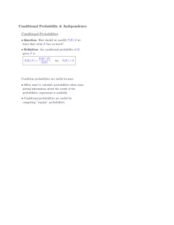
Review of Conditional Probability and Independence Definition L7.3 - PowerPoint PPT Presentation

Review of Conditional Probability and Independence Definition L7.3 (Def 1.3.2 on p.20): If A, B ∈ S and P ( B ) > 0 , then P ( A | B ) = P ( A ∩ B ) . P ( B ) Bayes’ Rule Theorem L7.2 (Thm 1.3.5 on p.23): Let A 1 , A 2 , . . . be a partition of the sample space S and B ⊂ S . If P ( B ) > 0 and P ( A i ) > 0 , then P ( B | A i ) P ( A i ) P ( A i | B ) = . � P ( B | A j ) P ( A j ) j : P ( A j ) > 0 19 / 25 Lecture 7: Methods of Estimation

Review of Conditional Probability and Independence Definition L7.4 (Def 4.2.1 on p.148): Let ( X, Y ) be a discrete bivariate random vector with joint pmf f ( x, y ) and marginal pmfs f X ( x ) and f Y ( y ) . For any x such that P ( X = x ) = f X ( x ) > 0 , the conditional pmf of Y given that X = x is the function of y defined by f ( y | x ) = P ( Y = y | X = x ) = f ( x, y ) f X ( x ) . For any y such that P ( Y = y ) = f Y ( y ) > 0 , the conditional pmf of X given that Y = y is the function of x defined by f ( x | y ) = P ( X = x | Y = y ) = f ( x, y ) f Y ( y ) . If g ( Y ) is a function of a discrete random variable Y , then the conditional expected value of g ( Y ) given that X = x is � E ( g ( Y ) | x ) = g ( y ) f ( y | x ) . y 20 / 25 Lecture 7: Methods of Estimation

Review of Conditional Probability and Independence Definition L7.5 (Def 4.2.3 on p.150): Let ( X, Y ) be a continuous bivariate random vector with joint pdf f ( x, y ) and marginal pdfs f X ( x ) and f Y ( y ) . For any x such that f X ( x ) > 0 , the conditional pdf of Y given that X = x is the function of y defined by f ( y | x ) = f ( x, y ) f X ( x ) . For any y such that f Y ( y ) > 0 , the conditional pdf of X given that Y = y is the function of x defined by f ( x | y ) = f ( x, y ) f Y ( y ) . If g ( Y ) is a function of a continuous random variable Y , then the conditional expected value of g ( Y ) given that X = x is � ∞ E ( g ( Y ) | x ) = g ( y ) f ( y | x ) dy. −∞ 21 / 25 Lecture 7: Methods of Estimation

Bayesian Estimation The Bayesian approach differs greatly from the classical approach that we have been discussing. In the Bayesian approach, the parameter θ is assumed to be a random variable/vector with prior distribution π ( θ ) . Then we can find update the pdf/pmf of the distribution of θ given data X = x using Bayes’ Rule π ( θ | x ) = f ( x , θ ) m ( x ) = f ( x | θ ) π ( θ ) m ( x ) where m ( x ) is the pdf/pmf of the marginal distribution of X . The updated prior is referred to as the posterior distribution . The Bayes estimator of θ is obtained by finding the mean of the posterior distribution; that is, ˆ θ B = E [ θ | X ] . 22 / 25 Lecture 7: Methods of Estimation

Bayesian Estimation Example L7.7 : Let X 1 , . . . , X n be a random sample from a Bernoulli( p ) distribution. Find the Bayes estimator of p , assuming that the prior distribution on p is beta( α , β ). Answer to Example L7.7 : Since X 1 , . . . , X n are iid Bernoulli( p ) random variables, � n i =1 X i is binomial( n , p ). The posterior distribution of p | � n i =1 X i = x is f ( x | p ) π ( p ) π ( p | x ) = m ( x ) p x (1 − p ) n − x Γ( α + β ) � n � Γ( α )Γ( β ) p α − 1 (1 − p ) β − 1 x = � 1 p x (1 − p ) n − x Γ( α + β ) � n Γ( α )Γ( β ) p α − 1 (1 − p ) β − 1 dp � 0 x p x + α − 1 (1 − p ) n − x + β − 1 = � 1 0 p x + α − 1 (1 − p ) n − x + β − 1 dp Γ( n + α + β ) Γ( x + α )Γ( n − x + β ) p x + α − 1 (1 − p ) n − x + β − 1 I (0 , 1) ( p ) . = 23 / 25 Lecture 7: Methods of Estimation

Bayesian Estimation Answer to Example L7.7 continued : Thus, p | � n i =1 X i = x follows a beta( � n i =1 x i + α , n − � n i =1 x i + β ) distribution. The Bayes estimator (posterior mean) is � n i =1 X i + α ˆ = p B α + β + n � � n � � α + β � n i =1 X i α = + α + β . α + β + n α + β + n n The Bayes estimator is a weighted average of ¯ X (the sample α mean based on the data) and E [ p ] = α + β (the mean of the prior distribution). 24 / 25 Lecture 7: Methods of Estimation

Bayesian Estimation Definition L7.6 (Def 7.2.15 on p.325): Let F denote the class of pdfs or pmfs f ( x | θ ) (indexed by θ ). A class Π of prior distributions is a conjugate family for F if the posterior distribution is in the class Π for all f ∈ F , all priors in Π , and all x ∈ X . As seen in Example L7.7, the beta family is conjugate for the binomial family. 25 / 25 Lecture 7: Methods of Estimation

Bayesian Tests Hypothesis testing is much different from a Bayesian perspective where the parameter is considered random. From the Bayesian perspective, the natural approach is to compute � P ( H 0 is true | x ) = P ( θ ∈ Θ 0 | x ) = π ( θ | x ) dθ Θ 0 and � P ( H 1 is true | x ) = P ( θ ∈ Θ c 0 | x ) = π ( θ | x ) dθ Θ c 0 based on the posterior distribution π ( θ | x ) . 7 / 14 Lecture 14: More Hypothesis Testing Examples

Bayesian Tests Example L14.2 : Suppose we toss a coin 5 times and count the total number of heads which occur. We assume each toss is independent and the probability of heads (denoted by p ) is the same on each toss. Consider a Bayesian model which assumes that p follows a Uniform (0 , 1) prior. What is the probability of the the null 5 � hypothesis H 0 : p ≤ . 5 if X i = 5 ? i =1 Answer to Example L14.2 : Since p | X = x ∼ beta ( � 5 i =1 x i + 1 , 5 − � 5 i =1 x i + 1) from slide 7.24, the probability is � . 5 � 5 � � 6 p 5 dp = 1 / 64 = . 015625 . � P p ≤ . 5 x i = 5 = � � 0 i =1 8 / 14 Lecture 14: More Hypothesis Testing Examples

Finding a Bayesian Credible Interval Interval estimators are much different from a Bayesian perspective where the parameter is considered random. Definition L16.5 (p.436): If π ( θ | x ) is the posterior distribution of θ given X = x , then for any set A ⊂ Θ , the credible probability of A is � P ( θ ∈ A | x ) = π ( θ | x ) dθ (assuming θ | x is continuous) A and A is a credible set for θ . 23 / 24 Lecture 16: Confidence Intervals

Finding a Bayesian Credible Interval Example L16.5 : Suppose X 1 , . . . , X n are iid Bernoulli( p ) random variables and suppose we consider a Bayesian model which assumes that p follows a Uniform (0 , 1) prior. Find a 90% credible set for p for the data set with 4 successes and 14 failures. Answer to Example L16.5 : From slide 7.23, p | � n i =1 X i = y ∼ beta ( y + α, n − y + β ) , we have p | X = x ∼ beta (4 + 1 = 5 , 14 + 1 = 15) . � p L So we can find p L such that π ( p | x ) dθ = . 05 and p U such 0 � 1 p U π ( p | x ) dθ = . 05 where π ( p | x ) = 58140 p 4 (1 − p ) 14 . that Using the R commands qbeta(.05,5,15) and qbeta(.95,5,15) , we obtain the 90% credible set ( . 1099 , . 4191) . The shortest 90% credible set ( . 0953 , . 3991) can be obtained with the R commands alpha=.02931685;qbeta(c(alpha,.9+alpha),5,15) since > dbeta(qbeta(c(alpha,.9+alpha),5,15),5,15) [1] 1.180588 1.180588 24 / 24 Lecture 16: Confidence Intervals