A Fresh Look at the Bayes Theorem from Information Theory Tan - PowerPoint PPT Presentation
A Fresh Look at the Bayes Theorem from Information Theory Tan Bui-Thanh Computational Engineering and Optimization (CEO) Group Department of Aerospace Engineering and Engineering Mechanics Institute for Computational Engineering and Sciences
A Fresh Look at the Bayes’ Theorem from Information Theory Tan Bui-Thanh Computational Engineering and Optimization (CEO) Group Department of Aerospace Engineering and Engineering Mechanics Institute for Computational Engineering and Sciences (ICES) The University of Texas at Austin Babuska Series, ICES Sep 9, 2016 (CEO Group UT Austin) Bayes’ Theorem Bayesian Inversions 1 / 28
Outline Bayesian Inversion Framework 1 Entropy 2 Relative Entropy 3 Bayes’ Theorem and Information Theory 4 Conclusions 5 (CEO Group UT Austin) Bayes’ Theorem Bayesian Inversions 2 / 28
Large-scale computation under uncertainty Inverse electromagnetic scattering Randomness Random errors in measurements are unavoidable Inadequacy of the mathematical model (Maxwell equations) Challenge How to invert for the invisible shape/medium using computational � 10 6 � electromagnetics with O degree of freedoms? (CEO Group UT Austin) Bayes’ Theorem Bayesian Inversions 3 / 28
Large-scale computation under uncertainty Full wave form seismic inversion Randomness Random errors in seismometer measurements are unavoidable Inadequacy of the mathematical model (elastodynamics) Challenge How to image the earth interior using forward computational model with � 10 9 � with O degree of freedoms? (CEO Group UT Austin) Bayes’ Theorem Bayesian Inversions 4 / 28
Inverse Shape Electromagnetic Scattering Problem Maxwell Equations: r ⇥ E = � µ @ H @ t , (Faraday) r ⇥ H = ✏@ E @ t , (Ampere) E : Electric field, H : Magnetic field, µ : permeability, ✏ : permittivity (CEO Group UT Austin) Bayes’ Theorem Bayesian Inversions 5 / 28
Inverse Shape Electromagnetic Scattering Problem Maxwell Equations: r ⇥ E = � µ @ H @ t , (Faraday) r ⇥ H = ✏@ E @ t , (Ampere) E : Electric field, H : Magnetic field, µ : permeability, ✏ : permittivity Forward problem (discontinuous Galerkin discretization) d = G ( x ) where G maps shape parameters x to electric/magnetic field d at the measurement points (CEO Group UT Austin) Bayes’ Theorem Bayesian Inversions 5 / 28
Inverse Shape Electromagnetic Scattering Problem Maxwell Equations: r ⇥ E = � µ @ H @ t , (Faraday) r ⇥ H = ✏@ E @ t , (Ampere) E : Electric field, H : Magnetic field, µ : permeability, ✏ : permittivity Forward problem (discontinuous Galerkin discretization) d = G ( x ) where G maps shape parameters x to electric/magnetic field d at the measurement points Inverse Problem Given (possibly noise-corrupted) measurements on d , infer x ? (CEO Group UT Austin) Bayes’ Theorem Bayesian Inversions 5 / 28
The Bayesian Statistical Inversion Framework (CEO Group UT Austin) Bayes’ Theorem Bayesian Inversions 6 / 28
The Bayesian Statistical Inversion Framework (CEO Group UT Austin) Bayes’ Theorem Bayesian Inversions 6 / 28
The Bayesian Statistical Inversion Framework Bayes Theorem ⇡ post ( x | d ) / ⇡ like ( d | x ) ⇥ ⇡ prior ( x ) (CEO Group UT Austin) Bayes’ Theorem Bayesian Inversions 6 / 28
Bayes theorem for inverse electromagnetic scattering Prior knowledge: The obstacle is smooth: Z 2 π ✓ ◆ ⇡ pr ( x ) / exp � � r 00 ( x ) d ✓ 0 (CEO Group UT Austin) Bayes’ Theorem Bayesian Inversions 7 / 28
Bayes theorem for inverse electromagnetic scattering Prior knowledge: The obstacle is smooth: Z 2 π ✓ ◆ ⇡ pr ( x ) / exp � � r 00 ( x ) d ✓ 0 Likelihood: Additive Gaussian noise, for example, ✓ ◆ � 1 2 k G ( x ) � d k 2 ⇡ like ( d | x ) / exp C noise (CEO Group UT Austin) Bayes’ Theorem Bayesian Inversions 7 / 28
Outline Bayesian Inversion Framework 1 Entropy 2 Relative Entropy 3 Bayes’ Theorem and Information Theory 4 Conclusions 5 (CEO Group UT Austin) Bayes’ Theorem Bayesian Inversions 8 / 28
Entropy Definition We define the uncertainty in a random variable X distributed by 0 ⇡ ( x ) 1 as Z H ( X ) = � ⇡ ( x ) log ⇡ ( x ) dx � 0 (CEO Group UT Austin) Bayes’ Theorem Bayesian Inversions 9 / 28
Entropy (CEO Group UT Austin) Bayes’ Theorem Bayesian Inversions 10 / 28
Entropy Wiener and Shannon Kolmogorov Copied from Sergio Verdu (CEO Group UT Austin) Bayes’ Theorem Bayesian Inversions 10 / 28
Entropy Wiener and Shannon Kolmogorov Copied from Sergio Verdu Wiener: “...for it belongs to the two of us equally” (CEO Group UT Austin) Bayes’ Theorem Bayesian Inversions 10 / 28
Entropy Wiener and Shannon Kolmogorov Copied from Sergio Verdu Wiener: “...for it belongs to the two of us equally” Shannon: “...a mathematical pun” (CEO Group UT Austin) Bayes’ Theorem Bayesian Inversions 10 / 28
Entropy Wiener and Shannon Kolmogorov Copied from Sergio Verdu Wiener: “...for it belongs to the two of us equally” Shannon: “...a mathematical pun” Kolmogorov: “...has no physical interpretation” (CEO Group UT Austin) Bayes’ Theorem Bayesian Inversions 10 / 28
Entropy Entropy of uniform distribution (CEO Group UT Austin) Bayes’ Theorem Bayesian Inversions 11 / 28
Entropy Entropy of uniform distribution Let U be a uniform random variable with values in X , and | X | < 1 (CEO Group UT Austin) Bayes’ Theorem Bayesian Inversions 11 / 28
Entropy Entropy of uniform distribution Let U be a uniform random variable with values in X , and | X | < 1 ⇡ ( u ) := 1 | X | ) H ( U ) = log ( | X | ) (CEO Group UT Austin) Bayes’ Theorem Bayesian Inversions 11 / 28
Entropy Entropy of uniform distribution Let U be a uniform random variable with values in X , and | X | < 1 ⇡ ( u ) := 1 | X | ) H ( U ) = log ( | X | ) How uncertain is the uniform random variable? (CEO Group UT Austin) Bayes’ Theorem Bayesian Inversions 11 / 28
Entropy Entropy of uniform distribution Let U be a uniform random variable with values in X , and | X | < 1 ⇡ ( u ) := 1 | X | ) H ( U ) = log ( | X | ) How uncertain is the uniform random variable? H ( X ) H ( U ) (CEO Group UT Austin) Bayes’ Theorem Bayesian Inversions 11 / 28
100 years of uniform distribution source: Christoph Aistleitner (CEO Group UT Austin) Bayes’ Theorem Bayesian Inversions 12 / 28
100 years of uniform distribution source: Christoph Aistleitner Hermann Weyl (CEO Group UT Austin) Bayes’ Theorem Bayesian Inversions 12 / 28
and Maximum entropy Maximum entropy distribution X with known mean and variance (CEO Group UT Austin) Bayes’ Theorem Bayesian Inversions 13 / 28
and Maximum entropy Maximum entropy distribution X with known mean and variance ⇡ ( x )? with maximum entropy (CEO Group UT Austin) Bayes’ Theorem Bayesian Inversions 13 / 28
and Maximum entropy Maximum entropy distribution X with known mean and variance ⇡ ( x )? with maximum entropy Z max π ( x ) H ( X ) = � ⇡ ( x ) log( ⇡ ( x )) dx subject to Z x ⇡ ( x ) dx = µ Z ( x � µ ) 2 ⇡ ( x ) dx = � 2 Z ⇡ ( x ) dx = 1 (CEO Group UT Austin) Bayes’ Theorem Bayesian Inversions 13 / 28
Gaussian and Maximum entropy Maximum entropy distribution X with known mean and variance ⇡ ( x )? with maximum entropy Z max π ( x ) H ( X ) = � ⇡ ( x ) log( ⇡ ( x )) dx subject to Z x ⇡ ( x ) dx = µ Z ( x � µ ) 2 ⇡ ( x ) dx = � 2 Z ⇡ ( x ) dx = 1 � µ, � 2 � Gaussian distribution: ⇡ ( x ) = N (CEO Group UT Austin) Bayes’ Theorem Bayesian Inversions 13 / 28
Outline Bayesian Inversion Framework 1 Entropy 2 Relative Entropy 3 Bayes’ Theorem and Information Theory 4 Conclusions 5 (CEO Group UT Austin) Bayes’ Theorem Bayesian Inversions 14 / 28
Relative Entropy Abraham Wald (1945) Harold Je ff reys (1945) Z ✓ ⇡ ( x ) ◆ D ( ⇡ || q ) := ⇡ ( x ) log dx q ( x ) (CEO Group UT Austin) Bayes’ Theorem Bayesian Inversions 15 / 28
Kullback-Leibler divergence = Relative Entropy Solomon Kullback Richard Leibler (1951) (1951) ✓ ⇡ ( x ) ◆ Z D ( ⇡ || q ) := ⇡ ( x ) log dx q ( x ) (CEO Group UT Austin) Bayes’ Theorem Bayesian Inversions 16 / 28
Kullback-Leibler divergence = Relative Entropy Solomon Kullback Richard Leibler (1951) (1951) ✓ ⇡ ( x ) ◆ ✓ ⇡ i ◆ Z X dx discrete D ( ⇡ || q ) := ⇡ ( x ) log = ⇡ i log q ( x ) q i (CEO Group UT Austin) Bayes’ Theorem Bayesian Inversions 16 / 28
Information Inequality The most important inequality in information theory D ( ⇡ || q ) � 0 Can we see it easily? (CEO Group UT Austin) Bayes’ Theorem Bayesian Inversions 17 / 28
Information Inequality The most important inequality in information theory D ( ⇡ || q ) � 0 Can we see it easily? (CEO Group UT Austin) Bayes’ Theorem Bayesian Inversions 17 / 28
Outline Bayesian Inversion Framework 1 Entropy 2 Relative Entropy 3 Bayes’ Theorem and Information Theory 4 Conclusions 5 (CEO Group UT Austin) Bayes’ Theorem Bayesian Inversions 18 / 28
From Relative Entropy to Bayes’ Theorem Toss n times an k th dimensional dice with the prior distribution of k X each face { p i } k i =1 : p i = 1 i =1 (CEO Group UT Austin) Bayes’ Theorem Bayesian Inversions 19 / 28
Recommend
More recommend
Explore More Topics
Stay informed with curated content and fresh updates.
