Bayesian Inference Harvard Math Camp - Econometrics Ashesh - PowerPoint PPT Presentation
Bayesian Inference Harvard Math Camp - Econometrics Ashesh Rambachan Summer 2018 Outline What is Bayesian Inference? Inference Frequentists vs. Bayesians Conjugate Priors Normal-Normal Beta-Bernoulli Multinomial-Dirichlet Exchangeability
Bayesian Inference Harvard Math Camp - Econometrics Ashesh Rambachan Summer 2018
Outline What is Bayesian Inference? Inference Frequentists vs. Bayesians Conjugate Priors Normal-Normal Beta-Bernoulli Multinomial-Dirichlet Exchangeability
Outline What is Bayesian Inference? Inference Frequentists vs. Bayesians Conjugate Priors Normal-Normal Beta-Bernoulli Multinomial-Dirichlet Exchangeability
Outline What is Bayesian Inference? Inference Frequentists vs. Bayesians Conjugate Priors Normal-Normal Beta-Bernoulli Multinomial-Dirichlet Exchangeability
Statistical Inference Observe data x i for i = 1 , . . . , n . ◮ Assume the data from from a random experiment, modeled by r.v. X with support X . ◮ { x i } n i =1 are realizations of X . ◮ Wish to use the data to learn something about F X ( x ) A statistical model is a set of probability distributions indexed by a parameter set. F = { P θ ( x ) : x ∈ X , θ ∈ Θ } ◮ Parametric if P can be indexed with a finite dimensional parameter set. Otherwise, non-parametric . Observe { x i } n i =1 and wish to make inferences about θ .
Statistical Models: Examples Example:the set of normal distributions with variance equal to one. Then, X = R , Θ = R and 1 e − 1 2 ( x − θ ) 2 . f θ ( x ) = √ 2 π Wish to learn about θ .
Outline What is Bayesian Inference? Inference Frequentists vs. Bayesians Conjugate Priors Normal-Normal Beta-Bernoulli Multinomial-Dirichlet Exchangeability
Frequentists vs. Bayesians Suppose we have a ”good” statistical model. F X ( x ) ∈ F and there exists some θ ∗ ∈ Θ such that F X ( x ) = F θ ∗ ( x ) The whole point of statistical inference is that θ ∗ is unknown. ◮ How should we model an unknown θ ∗ and how does that choice affect how inference should be conducted.
Frequentists Even though θ ∗ is unknown, we should view it as fixed . The data are modeled as random variables X 1 , . . . , X n drawn from the fixed, unknown distribution F θ ∗ ( x ). The random experiment is: 1. Nature draws the data x 1 , . . . , x n from F θ ∗ ( x ). 2. We observe x 1 , . . . , x n and plugs them into our estimator, θ ( · ). Our estimate is ˆ ˆ θ ( x 1 , . . . , x n ).
Frequentists Freqentists engage in the following thought experiment: ◮ Repeat the experiment many times. Each time, we obtain new data x b 1 , . . . , x b n and construct a new estimate, ˆ n ) = ˆ θ ( x b 1 , . . . , x b θ b . ◮ What properties will the sampling distribution of my estimator have? ◮ As n → ∞ , what properties will the distribution of of my estimator have? Frequentists focuses on the behavior of estimators in a repeated random experiment , where we want to understand the properties of ˆ θ ( · ) under the sampling distribution of the data.
Bayesians Bayesians, model the unknown θ ∗ as a random variable itself, with its own distriution, Π( θ ). This is the prior distribution . ◮ The prior encodes prior information about the parameter θ available prior to observing the data. This may come from prior experiments, observational studies or economic theory.
Bayesians The random experiment then has an extra step: 1. Nature draws θ ∗ from the prior, Π( θ ). This is unobserved. 2. Nature draws realizations x 1 , . . . , x n from the distribution F θ ∗ ( x ). These are the data. 3. We observes x 1 , . . . , x n and plugs them into our estimator, θ ( · ). Her estimate is ˆ ˆ θ ( x 1 , . . . , x n ).
Bayesians What is the point of the prior? Bayes’ rule . ◮ Provides a logically consistent rule for combining prior information with the observed data. ◮ x = ( x 1 , . . . , x n ) and f θ ( x ) is the density associated with distribution F θ ( x ) and π ( θ ) is defined analogously. π ( θ | x ) = f θ ( x ) π ( θ ) f ( x ) ◮ marginal density of X : f ( x ) = � Θ f θ ( x ) π ( θ ) d θ ◮ likelihood function : f θ ( x ) ◮ posterior density : π ( θ | x ) The posterior distribution of θ | x is the central object of interest in Bayesian inference.
Bayesians: Brief Aside You will often see Bayes’ rule written as π ( θ | x ) ∝ f θ ( x ) π ( θ ) In English Bayes’ rule says, ”the posterior is proportional to the likelihood times the prior.”
Bayesians Uses the posterior distribution to make inferences about θ . ◮ E.g. the ”posterior expectation of θ given the data x ” E [ θ | x ] . is a common object of interest. ◮ Could also compute Med ( θ | X ) , P ( θ < ˜ θ | X ) and so on. The posterior density, x is fixed at its realized value and θ varies over Θ. ◮ In this sense, bayesian inference is completely conditional on the observed data .
Bayesians Completely swept under the rug the very important question: How do we choose a prior distribution? ◮ Short answer: it’s not easy! Requires a lot of careful thought. ◮ We’ll pick this issue up at times in Ec 2120. ◮ If interested, check out Kasy & Fessley (2018) - “how should economic theory guide the choice of priors?”
Outline What is Bayesian Inference? Inference Frequentists vs. Bayesians Conjugate Priors Normal-Normal Beta-Bernoulli Multinomial-Dirichlet Exchangeability
Conjugate Priors Once we have a prior distribution and a likelihood function, the only computational step is to use Bayes’ rule. ◮ Sounds simple... But this can often be a mess. ◮ Lots of Bayesian statistics focues on doing this in a computationally feasible manner - MCMC, Variational Inference. Important tool in bayesian inference: conjugate priors . ◮ Prior distribution is conjugate for a given likelihood function if the associated posterior distribution is in the same family of distributions as the prior. We’ll cover three useful conjugate priors that you will encounter.
Outline What is Bayesian Inference? Inference Frequentists vs. Bayesians Conjugate Priors Normal-Normal Beta-Bernoulli Multinomial-Dirichlet Exchangeability
The data The data are X = ( X 1 , . . . , X n ).Conditional on θ , X i are i.i.d. with X i ∼ N ( µ, σ 2 ) ◮ σ 2 is fixed and assumed known. ◮ Define the precision as λ σ = 1 /σ 2 . ◮ The parameter space is θ = R . We observe realizations x = ( x 1 , . . . , x n ).
The likelihood The likelihood function is f µ ( x ) = f ( x | µ ) = Π n i =1 f ( x i | µ ) i =1 exp( − 1 2 λ σ ( x i − µ ) 2 ) ∝ Π n n ∝ exp( − 1 � ( x i − µ ) 2 ) 2 λ σ i =1
The prior The prior distribution for µ is also normal. We assume that µ ∼ N ( m , τ 2 ) . ◮ Useful to define the prior precision as λ τ = 1 /τ 2 . So, π ( µ ) ∝ exp( − 1 2 λ τ ( µ − m ) 2 )
The posterior The posterior distribution is given by Bayes’ rule. This is a pain in the butt but the result is really nice. *Takes a deep breath*
The posterior π ( µ | x ) ∝ f µ ( x ) π ( µ ) n ∝ exp( − 1 ( x i − µ ) 2 ) exp( − 1 � 2 λ τ ( µ − m ) 2 ) 2 λ σ i =1 n − λ σ i − 2 x i µ + µ 2 ) − λ τ � 2 ( µ 2 − 2 µ m + m 2 ) � � ( x 2 ∝ exp 2 i =1 � n − n λ σ + λ τ µ 2 + λ σ i =1 x i + λ τ m � � ∝ exp µ 2 2 � n − n λ σ + λ τ ( µ 2 − λ σ i =1 x i + λ τ m � � ∝ exp µ ) 2 n λ σ + σ τ − n λ σ + λ τ ( µ 2 − n λ σ ¯ x + λ τ m � � ∝ exp µ ) 2 n λ σ + λ τ − n λ σ + λ τ ( µ 2 − n λ σ ¯ x + λ τ m µ + ( n λ σ ¯ x + λ τ m � � ) 2 ) ∝ exp 2 n λ σ + λ τ n λ σ + λ τ
The posterior So, − n λ σ + λ τ ( µ − n λ σ ¯ x + λ τ m � ) 2 � π ( µ | x ) ∝ exp 2 n λ σ + λ τ and µ | x ∼ N ( n λ σ ¯ x + λ τ m , n λ σ + λ τ ) . n λ σ + λ τ
The posterior As I said: This was a pain in the butt. Is there an easier way? Yes! Use our results for the multivariate normal distribution. X | µ ∼ N ( µ, σ 2 I n ) . Can show that the marginal distribution of X is given X ∼ N ( m , ( σ 2 + τ 2 ) I n ) and that the joint distribution of X , µ is given by � ( σ 2 + τ 2 ) I n τ 2 l � X � � m � � ∼ N ( , τ 2 l ′ τ 2 µ m where l is a n × 1 vector of ones.
The posterior It then follows that τ 2 σ 2 + τ 2 l ′ I n ( x − m ) , τ 2 − τ 2 ( σ 2 + τ 2 ) − 1 τ 2 l ′ l ) . µ | X = x ∼ N ( m + Exactly as before!
The posterior Posterior mean: E [ µ | x ] = n λ σ ¯ x + λ τ m n λ σ + λ τ Posterior precision: ¯ λ τ = n λ σ + λ τ Interpretation: ◮ Posterior mean is a weighted average of the sample mean and the prior mean in which the weights are the precisions. ◮ If λ τ is large and the prior has a low variance, the prior mean receives a larger weight. ◮ ”Shrinking” the posterior mean towards the prior
Machine learning aside Machine learning aside: ǫ i | X , β ∼ N (0 , σ 2 ) i . i . d . Y i = X i β + ǫ i , β | X ∼ N (0 , Ω) Joint likelihood of Y , β gives a ridge-type objective ∝ − 1 ( Y i − β X i ) 2 − 1 � 2 β ′ Ω β 2 σ 2 i Maximum a posteriori estimator: Ridge regression. Can similarly motivate lasso using this Bayesian approach.
Outline What is Bayesian Inference? Inference Frequentists vs. Bayesians Conjugate Priors Normal-Normal Beta-Bernoulli Multinomial-Dirichlet Exchangeability
Recommend
More recommend
Explore More Topics
Stay informed with curated content and fresh updates.
