CS 287 Lecture 11 (Fall 2019) Probability Review, Bayes Filters, - PowerPoint PPT Presentation
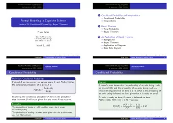
CS 287 Lecture 11 (Fall 2019) Probability Review, Bayes Filters, Gaussians Pieter Abbeel UC Berkeley EECS Many slides adapted from Thrun, Burgard and Fox, Probabilistic Robotics Outline n Probability Review n Bayes Filters n Gaussians Why
CS 287 Lecture 11 (Fall 2019) Probability Review, Bayes Filters, Gaussians Pieter Abbeel UC Berkeley EECS Many slides adapted from Thrun, Burgard and Fox, Probabilistic Robotics
Outline n Probability Review n Bayes Filters n Gaussians
Why probability in robotics? n Often the state of the robot and of its environment are unknown and only noisy sensors are available n Probability provides a framework to fuse sensory information à Result: probability distribution over possible states of robot and environment n Dynamics is often stochastic, hence can’t optimize for a particular outcome, but only optimize to obtain a good distribution over outcomes n Probability provides a framework to reason in this setting à Ability to find good control policies for stochastic dynamics and environments
Example 1: Helicopter State: position, orientation, velocity, angular rate n Sensors: n n GPS : noisy estimate of position (sometimes also velocity) n Inertial sensing unit: noisy measurements from 3-axis gyro [=angular rate sensor], (i) (ii) 3-axis accelerometer [measures acceleration + gravity; e.g., measures (0,0,0) in free-fall], (iii) 3-axis magnetometer Dynamics: n n Noise from: wind, unmodeled dynamics in engine, servos, blades
Example 2: Mobile robot inside building State: position and heading n Sensors: n n Odometry (=sensing motion of actuators): e.g., wheel encoders n Laser range finder: n Measures time of flight of a laser beam between departure and return n Return is typically happening when hitting a surface that reflects the beam back to where it came from n Dynamics: n Noise from: wheel slippage, unmodeled variation in floor
Outline n Probability Review n Bayes Filters n Gaussians
Axioms of Probability Theory £ £ 0 Pr( A ) 1 Pr( φ ) = 0 Pr( Ω ) = 1 Pr( A ∪ B ) = Pr( A ) + Pr( B ) − Pr( A ∩ B ) Pr (A) denotes probability that the outcome ω is an element of the set of possible outcomes A . A is often called an event. Same for B. Ω is the set of all possible outcomes. ϕ is the empty set.
Using the Axioms Pr( A ∪ ( Ω \ A )) Pr( A ) + Pr( Ω \ A ) − Pr( A ∩ ( Ω \ A )) = Pr( Ω ) Pr( A ) + Pr( Ω \ A ) − Pr( φ ) = 1 Pr( A ) + Pr( Ω \ A ) − 0 = Pr( Ω \ A ) 1 − Pr( A ) =
Discrete Random Variables Ω x 2 x 3 x 1 x 4 X denotes a random variable. n X can take on a countable number of values in {x 1 , x 2 , …, x n }. n P(X=x i ) , or P(x i ) , is the probability that the random variable X takes n on value x i . P(.) is called probability mass function. n E.g., X models the outcome of a coin flip, x 1 = head, x 2 = tail, P( x 1 ) n = 0.5 , P( x 2 ) = 0.5
Continuous Random Variables X takes on values in the continuum. n p(X=x) , or p(x) , is a probability density function. n b ò Î = Pr( x ( a , b )) p ( x ) dx a p(x) E.g. n x
Joint and Conditional Probability P(X=x and Y=y) = P(x,y) n X and Y are independent iff n P(x,y) = P(x) P(y) P(x | y) is the probability of x given y n P(x | y) = P(x,y) / P(y) P(x,y) = P(x | y) P(y) If X and Y are independent then n P(x | y) = P(x) Same for probability densities, just P à p n
Law of Total Probability, Marginals Discrete case Continuous case å ò = = 1 P ( x ) 1 p ( x ) dx x å ò = = P ( x ) P ( x , y ) p ( x ) p ( x , y ) dy y å ò = = P ( x ) P ( x | y ) P ( y ) p ( x ) p ( x | y ) p ( y ) dy y
Bayes Rule = = P ( x , y ) P ( x | y ) P ( y ) P ( y | x ) P ( x ) Þ × P ( y | x ) P ( x ) likelihood prior = = P ( x y ) P ( y ) evidence
Normalization P ( y | x ) P ( x ) = = h P ( x y ) P ( y | x ) P ( x ) P ( y ) 1 - h = 1 = P ( y ) å P ( y | x ) P ( x ) x Algorithm: " = x : aux P ( y | x ) P ( x ) x | y 1 h = å aux x | y x " = h x : P ( x | y ) aux x | y
Conditioning Law of total probability: n ò = P ( x ) P ( x , z ) dz ò = P ( x ) P ( x | z ) P ( z ) dz ò = P ( x y ) P ( x | y , z ) P ( z | y ) dz
Bayes Rule with Background Knowledge P ( y | x , z ) P ( x | z ) = P ( x | y , z ) P ( y | z )
Conditional Independence = P ( x , y z ) P ( x | z ) P ( y | z ) = equivalent to P ( x z ) P ( x | z , y ) = and P ( y z ) P ( y | z , x )
Simple Example of State Estimation Suppose a robot obtains measurement z n What is P(open|z)? n
Causal vs. Diagnostic Reasoning n P(open|z) is diagnostic. n P(z|open) is causal. count frequencies! n Often causal knowledge is easier to obtain. n Bayes rule allows us to use causal knowledge: P ( z | open ) P ( open ) = P ( open | z ) P ( z )
Example P(z| ¬ open) = 0.3 P(z|open) = 0.6 n P(open) = P( ¬ open) = 0.5 n P ( open | z ) = P ( z | open ) P ( open ) P ( z ) P ( z | open ) P ( open ) = P ( open | z ) + ¬ ¬ P ( z | open ) p ( open ) P ( z | open ) p ( open ) × 0 . 6 0 . 5 2 = = = P ( open | z ) 0 . 67 × + × 0 . 6 0 . 5 0 . 3 0 . 5 3 • z raises the probability that the door is open.
Combining Evidence n Suppose our robot obtains another observation z 2 . n How can we integrate this new information? n More generally, how can we estimate P(x| z 1 ...z n ) ?
Recursive Bayesian Updating P ( z | x , z , ! , z ) P ( x | z , ! , z ) - - n 1 n 1 1 n 1 = P ( x | z , ! , z ) 1 n P ( z | z , ! , z ) - n 1 n 1 Markov assumption : z n is independent of z 1 ,...,z n-1 if we know x. P ( x | z 1 , … , z n ) = P ( z n | x ) P ( x | z 1 , … , z n − 1 ) P ( z n | z 1 , … , z n − 1 ) = η P ( z n | x ) P ( x | z 1 , … , z n − 1 ) # & ∏ P ( z i | x ) ( P ( x ) = η 1... n % $ ' i = 1... n
Example: Second Measurement P(z 2 | ¬ open) = 0.6 P(z 2 |open) = 0.5 n P(open|z 1 )=2/3 n P ( z | open ) P ( open | z ) = 2 1 P ( open | z , z ) 2 1 + ¬ ¬ P ( z | open ) P ( open | z ) P ( z | open ) P ( open | z ) 2 1 2 1 1 2 × 5 2 3 = = = 0 . 625 1 2 3 1 8 × + × 2 3 5 3 • z 2 lowers the probability that the door is open.
A Typical Pitfall n Two possible locations 1 p(x2 | d) p(x1 | d) 0.9 x 1 and x 2 0.8 0.7 0.6 n P(x 1 )=0.99 p( x | d) 0.5 0.4 0.3 n P(z| x 2 )=0.09 0.2 0.1 P(z| x 1 )=0.07 0 5 10 15 20 25 30 35 40 45 50 Number of integrations If measurements are not independent but are treated as independent à can quickly end up overconfident
Outline n Probability Review n Bayes Filters n Gaussians
Actions n Often the world is dynamic since n actions carried out by the robot , n actions carried out by other agents , n or just the time passing by change the world. n How can we incorporate such actions ?
Typical Actions The robot turns its wheels to move n The robot uses its manipulator to grasp an object n Plants grow over time … n Actions are never carried out with absolute certainty . n In contrast to measurements, actions generally increase the n uncertainty .
Modeling Actions n To incorporate the outcome of an action u into the current “ belief ” , we use the conditional pdf P(x’|u,x) n This term specifies the pdf that executing u changes the state from x to x’ .
Example: Closing the door
State Transitions P(x’|u,x) for u = “close door”: 0.9 0.1 open closed 1 0 If the door is open, the action “close door” succeeds in 90% of all cases.
Integrating the Outcome of Actions Continuous case: ∫ P ( x ' | u ) = P ( x ' | u , x ) P ( x ) dx Discrete case: ∑ P ( x ' | u ) = P ( x ' | u , x ) P ( x )
Example: The Resulting Belief ∑ P ( closed | u ) = P ( closed | u , x ) P ( x ) = P ( closed | u , open ) P ( open ) + P ( closed | u , closed ) P ( closed ) = 9 10 ∗ 5 8 + 1 1 ∗ 3 8 = 15 16 ∑ P ( open | u ) = P ( open | u , x ) P ( x ) = P ( open | u , open ) P ( open ) + P ( open | u , closed ) P ( closed ) = 1 10 ∗ 5 8 + 0 1 ∗ 3 8 = 1 16 = 1 − P ( closed | u )
Measurements n Bayes rule P ( x z ) = P ( z | x ) P ( x ) = likelihood ⋅ prior P ( z ) evidence
Bayes Filters: Framework Given: n Stream of observations z and action data u: n = d { u , z ! , u , z } t 1 1 t t Sensor model P(z|x). n Action model P(x’|u,x) . n Prior probability of the system state P(x). n Wanted: n Estimate of the state X of a dynamical system. n = Bel ( x ) P ( x | u , z ! , u , z ) The posterior of the state is also called Belief : n t t 1 1 t t
Markov Assumption p ( z t | x 0: t , z 1: t − 1 , u 1: t ) = p ( z t | x t ) p ( x t | x 1: t − 1 , z 1: t − 1 , u 1: t ) = p ( x t | x t − 1 , u t ) Underlying Assumptions Static world n Independent noise n Perfect model, no approximation errors n
Recommend
More recommend
Explore More Topics
Stay informed with curated content and fresh updates.
