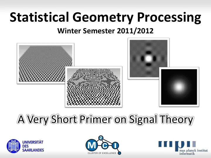
Statistical Geometry Processing Winter Semester 2011/2012 A Very - PowerPoint PPT Presentation

Statistical Geometry Processing Winter Semester 2011/2012 A Very Short Primer on Signal Theory

Topics Topics • Fourier transform • Theorems • Analysis of regularly sampled signals • Irregular sampling 2

Fourier Basis Fourier Basis • Function space: {𝑔: ℝ → ℝ, 𝑔 sufficiently smooth}  Fourier basis can represent – Functions of finite variation – Lipchitz-smooth functions • Basis: sine waves of different frequency and phase :  Real basis: {sin 2𝜌𝜕𝑦 , cos 2𝜌𝜕𝑦 𝜕 ∈ ℝ  Complex variant: {𝑓 −2𝜌𝑗𝜕𝑦 𝜕 ∈ ℝ (Euler‘s formula: 𝑓 𝑗𝑦 = cos 𝑦 + 𝑗 sin 𝑦 ) 3

Fourier Transform Fourier Basis properties: • Fourier basis: {𝑓 −𝑗2𝜌𝜕𝑦 𝜕 ∈ ℝ  Orthogonal basis  Projection via scalar products  Fourier transform • Fourier transform: (f: ℝ → ℂ) → F: ℝ → ℂ ∞ 𝑔 𝑦 𝑓 −2𝜌𝑗𝑦𝜕 𝑒𝑦 𝐺(𝜕) = −∞ • Inverse Fourier transform: F: ℝ → ℂ → (f: ℝ → ℂ) ∞ 𝐺 𝑦 𝑓 2𝜌𝑗𝑦𝜕 𝑒𝑦 𝑔(𝜕) = −∞ 4

Fourier Transform Interpreting the result: • Transforming a real function f: ℝ → ℝ • Result: F 𝜕 : ℝ → ℂ  𝜕 are frequencies (real) Im 𝜕 = 𝑓 −𝑗𝑦  Real input 𝑔 : Symmetric F −𝜕 = F 𝜕 𝜕 ∡𝜕  Output are complex numbers Re – Magnitude: “power spectrum” (frequency content) – Phase: phase spectrum (encodes shifts) 5

Important Functions Some important Fourier-transform pairs box( x ) sinc( 𝜕 ) • Box function: 𝑔 𝑦 = box 𝑦 → 𝐺 𝜕 = sin 𝜕 ≔ sinc 𝜕 𝜕 • Gaussian: 𝑏 ⋅ 𝑓 − 𝜌𝜕 2 𝜌 𝑔 𝑦 = 𝑓 −𝑏𝑦 2 → 𝐺 𝜕 = 𝑏 6

Higher Dimensional FT Multi-dimensional Fourier Basis: • Functions f: ℝ 𝑒 → ℂ • 2D Fourier basis: 𝑔(𝑦, 𝑧) represented as combination of {𝑓 −𝑗2𝜌𝜕 𝑦 𝑦 ⋅ 𝑓 −𝑗2𝜌𝜕 𝑧 𝑧 𝜕 𝑦 , 𝜕 𝑧 ∈ ℝ • In general: all combinations of 1D functions 7

Convolution Convolution: • Weighted average of functions g • Definition: f      f ( t ) g ( t ) f ( x ) g ( x t ) dx   t Example:   8 / 116 8

Theorems Fourier transform is an isometry: • 𝑔, 𝑕 = 𝐺, 𝐻 • In particular 𝑔 = 𝐺 Convolution theorem: • 𝐺𝑈 𝑔⨂𝑕 = 𝐺 ⋅ G • Fourier Transform converts convolution into multiplication  All other cases as well: 𝐺𝑈 −1 𝑔 ⋅ 𝑕 = 𝐺⨂G , 𝐺𝑈 𝑔 ⋅ 𝑕 = 𝐺⨂G , 𝐺𝑈 −1 𝐺 ⋅ 𝐻 = 𝐺⨂G  Fourier basis diagonalizes shift-invariant linear operators 9

Sampling a Signal Given: • Signal 𝑔: ℝ → ℝ • Store digitally:  Sample regularly … 𝑔 0.3 , 𝑔 0.4 , 𝑔 0.5 … • Question: what information is lost? 10

Sampling 11

Regular Sampling Results: Sampling • Band-limited signals can be represented exactly  Sampling with frequency 𝜉 𝑡 : Highest frequency in Fourier spectrum ≤ 𝜉 𝑡 /2 • Higher frequencies alias  Aliasing artifacts (low-frequency patterns)  Cannot be removed after sampling (loss of information) band-limited aliasing 12

Regular Sampling Result: Reconstruction • When reconstructing from discrete samples • Use band-limited basis functions  Highest frequency in Fourier spectrum ≤ 𝜉 𝑡 /2  Otherwise: Reconstruction aliasing 13

Regular Sampling Reconstruction Filters • Optimal filter: sinc (no frequencies discarded) • However:  Ringing artifacts in spatial domain  Not useful for images (better for audio) • Compromise  Gaussian filter (most frequently used)  There exist better ones, such as Mitchell-Netravalli, Lancos, etc... 2D sinc 2D Gaussian 14

Irregular Sampling Irregular Sampling • No comparable formal theory • However: similar idea  Band- limited by “sampling frequency”  Sampling frequency = mean sample spacing – Not as clearly defined as in regular grids – May vary locally (adaptive sampling) • Aliasing  Random sampling creates noise as aliasing artifacts  Evenly distributed sample concentrate noise in higher frequency bands in comparison to purely random sampling 15

Consequences for our applications When designing bases for function spaces • Use band-limited functions • Typical scenario:  Regular grid with spacing 𝜏  Grid points 𝐡 𝑗  Use functions: exp − 𝐲−𝐡 𝑗 2 𝜏 2 • Irregular sampling:  Same idea  Use estimated sample spacing instead of grid width  Set 𝜏 to average sample spacing to neighbors 16