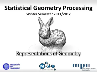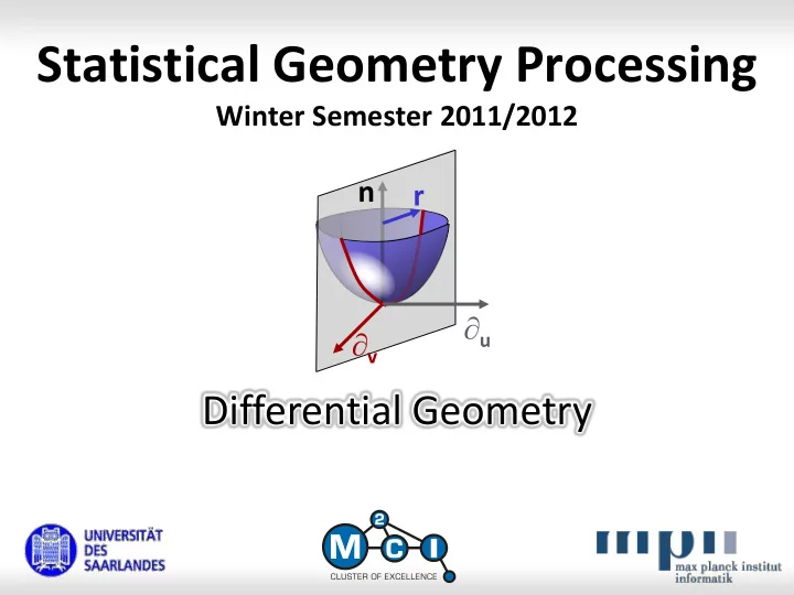
Statistical Geometry Processing Winter Semester 2011/2012 n r u - PowerPoint PPT Presentation

Statistical Geometry Processing Winter Semester 2011/2012 n r  u  v Differential Geometry

Multi-Dimensional Derivatives

Derivative of a Function Reminder: The derivative of a function is defined as   d f ( t h ) f ( t )  f ( t ) : lim dt h  h 0 If limit exists: function is called differentiable . Other notation: d k d    f ( t ) f ' ( t ) f ( t )  ( k ) f ( t ) f ( t )   dt k dt variable time from context variables repeated differentiation (higher order derivatives) 3

Taylor Approximation Smooth functions can be approximated locally:  f ( x ) f ( x ) • 0 d     f ( x ) x x 0 0 dx 2 1 d   2    f ( x ) x x ... 0 0 2 2 dx k 1 d   k  k 1    ... f ( x ) x x O ( x ) 0 0 k k ! dx • Convergence: holomorphic functions • Local approximation for smooth functions 4

Rule of Thumb Derivatives and Polynomials • Polynomial: 𝑔 𝑦 = 𝑑 0 + 𝑑 1 𝑦 + 𝑑 2 𝑦 2 + 𝑑 3 𝑦 3 …  0th-order derivative: 𝑔 0 = 𝑑 0  1st-order derivative: 𝑔′ 0 = 𝑑 1  2nd-order derivative: 𝑔′′ 0 = 2𝑑 2  3rd-order derivative: 𝑔′′′ 0 = 6𝑑 3  ... Rule of Thumb: • Derivatives correspond to polynomial coefficients • Estimate derivates  polynomial fitting 5

Differentiation is Ill-posed! h Regularization • Numerical differentiation needs regularization  Higher order is more problematic • Finite differences (larger h ) • Averaging (polynomial fitting) over finite domain 6

Partial Derivative Multivariate functions: • Notation changes: use curly-d   f ( x ,..., x , x , x ,..., x ) :   1 k 1 k k 1 n  x k   f ( x ,..., x , x h , x ,..., x ) f ( x ,..., x , x , x ,..., x ) 1 k  1 k k  1 n 1 k  1 k k  1 n lim h h  0 • Alternative notation:     f ( x ) f ( x ) f ( x ) k x  x k k 7

Special Cases Derivatives for: • Functions f :  n   (“heightfield”) • Functions f :    n (“curves”) • Functions f :  n   m (general case) 8

Special Cases Derivatives for: • Functions f :  n   (“heightfield”) • Functions f :    n (“curves”) • Functions f :  n   m (general case) 9

Gradient Gradient: • Given a function f :  n   (“heightfield”) • The vector of all partial derivatives of f is called the gradient :           f ( x )   x x     1 1        f ( x ) f ( x )         f ( x )           x x     n n 10

Gradient Gradient:     f ( x ) f ( x ) ( x x ) 0 0 0  f( x ) f( x ) f( x ) x 0 x x 1 x 1 x 2 x 2 • gradient: vector pointing in direction of steepest ascent. • Local linear approximation (Taylor):      f ( x ) f ( x ) f ( x ) ( x x ) 0 0 0 11

Higher Order Derivatives Higher order Derivatives:        ... f • Can do all combinations:      x x x   i i i 1 2 k • Order does not matter for f  C k 12

Hessian Matrix Higher order Derivatives: • Important special case: Second order derivative    2        2     x x x x    x 2 1 n 1 1      2      f ( x ) : H ( x )   2    x x x x   x f 1 2 n 2 1             2          2 x x x x  x   1 n 2 n n • “Hessian” matrix (symmetric for f  C 2 ) • Orthogonal Eigenbasis, full Eigenspectrum 13

Taylor Approximation f( x ) x 2nd order approximation x 1 (schematic) x 2 Second order Taylor approximation: • Fit a paraboloid to a general function 1        T    f ( x ) f ( x ) f ( x ) ( x x ) ( x x ) H ( x ) ( x x ) 0 0 0 0 f 0 0 2 14

Special Cases Derivatives for: • Functions f :  n   (“heightfield”) • Functions f :    n (“curves”) • Functions f :  n   m (general case) 15

Derivatives of Curves Derivatives of vector valued functions: • Given a function f :    n (“curve”)  f ( t )   1   f ( t )      f ( t )   n • We can compute derivatives for every output dimension:   d  f ( t )  1 dt   d     f ( t ) : : f ' ( t ) : f ( t )    dt d   f ( t )   n dt   16

Geometric Meaning f ( t ) t 0 f ’( t 0 ) Tangent Vector: • f ’: tangent vector . • Motion of physical particle: f = velocity. • Higher order derivatives: Again vector functions .. • Second derivative f = acceleration 17

Special Cases Derivatives for: • Functions f :  n   (“heightfield”) • Functions f :    n (“curves”) • Functions f :  n   m (general case) 18 / 76 18

You can combine it... General case: • Given a function f :  n   m (“space warp”)  f ( x ,..., x )   1 1 n      f ( x ) f ( x ,..., x )    1 n   f ( x ,..., x )   m 1 n • Maps points in space to other points in space • First derivative: Derivatives of all output components of f w.r.t. all input directions . • “Jacobian matrix”: denoted by  f or J f 19

Jacobian Matrix Jacobian Matrix:     f ( x ) J ( x ) f ( x ,..., x ) f 1 n      T   f ( x ,..., x ) f ( x ) f ( x )      1 1 n x 1 x 1 1 n                   T   f ( x ,..., x ) f ( x ) f ( x )      m 1 n x m x m 1 n Use in a first-order Taylor approximation:      f ( x ) f ( x ) J ( x ) x x 0 f 0 0 matrix / vector product 20

Coordinate Systems Problem: • What happens, if the coordinate system changes? • Partial derivatives go into different directions then. • Do we get the same result? 21

Total Derivative First order Taylor approx.:     f ( x ) f ( x ) ( x x ) 0 0 0      f ( x ) f ( x ) ( x x ) R ( x ) • 0 0 0 x f( x ) 0 x 0 • Converges for C 1 functions x 1 f :  n   m x 2 R ( x ) x  lim 0 , 0  x x  x x 0 0 (“ totally differentiable ”) 22

Partial Derivatives Consequences: • A linear function: fully determined by image of a basis • Hence: Directions of partial derivatives do not matter – this is just a basis transform.  We can use any linear independent set of directions T  Transform to standard basis by multiplying with T -1 • Similar argument for higher order derivatives 23

Directional Derivative The directional derivative is defined as: • Given f :  n   m and v   n , || v || = 1. • Directional derivative:  f d     f ( x ) ( x ) : f ( x t v ) v  v dt • Compute from Jacobian matrix v    f ( x ) f ( x ) v v (requires total differentiability) 24

Multi-Dimensional Optimization

Optimization Problems Optimization Problem: • Given a C 1 function f :  n   (general heightfield) • We are looking for a local extremum (minimum / maximum) of this function Theorem: • x is a local extremum   f ( x ) = 0 Sketch of a proof: If  f ( x )  0, we can walk a small step in gradient direction to improve the score further (in case of a maximum, minimum similar). 26

Critical Points Critical points: •  f ( x ) = 0 does not guarantee an extremum (saddle points) • Points with  f ( x ) = 0 are called critical points .  i > 0  0 > 0,  1 < 0 • Final decision via Hessian matrix :  All eigenvalues > 0: local minimum  All eigenvalues < 0: local maximum  Mixed eigenvalues: saddle point  0 = 0,  1 > 0  Some zero eigenvalues: critical line 27

Quadratic Optimization Quadratic Case: • f :  n   • Objective function: f ( x ) = x T A x + b T x + c  symmetric n  n matrix A  n -dim. vector b  constant c • Gradient:  f ( x ) = 2 A x + b • Critical points: solution to 2 A x = - b • Solution: Solve system of linear equations 28

Example Gradient computation example:  a   a             x , y ax by     b b      a b   x        2 2    x , y ax 2 bxy cy     b c y         2 ax 2 by  x  x     2 A       2 bx 2 cy y    y 29