Forty years of Quicksort and Quickselect: a personal view Conrado - PowerPoint PPT Presentation
Forty years of Quicksort and Quickselect: a personal view Conrado Martnez Univ. Politcnica de Catalunya, Spain Introduction Quicksort and quickselect were invented in the early sixties by C.A.R.
Small Subfiles •• ◦ • • • ◦ Using insertion sort with n 0 ≤ 10 reduces the average cost; the optimal choice for n 0 is 5 Selection (we locate the minimum, then the second minimum, etc.) reduces the average cost if n 0 ≤ 11 ; the optimum n 0 is 6 Optimized selection (looks for the m -th from the minimum or the maximum, whatever is closer) yields improved average performance if n 0 ≤ 22 ; the optimum n 0 is 11 17/51 Univ. Politècnica de Catalunya, Spain
Median-of-three •• ◦ • • ◦ In quicksort with median-of-three, the pivot of each recursive stage is selected as the median of a sample of three elements (Singleton, 1969) 18/51 Univ. Politècnica de Catalunya, Spain
Median-of-three •• ◦ • • ◦ In quicksort with median-of-three, the pivot of each recursive stage is selected as the median of a sample of three elements (Singleton, 1969) This reduces the probability of uneven partitions which lead to quadratic worst-case 18/51 Univ. Politècnica de Catalunya, Spain
Median-of-three •• ◦ • • ◦ We have in this case π n,k = ( k − 1)( n − k ) � n � 3 19/51 Univ. Politècnica de Catalunya, Spain
Median-of-three •• ◦ • • ◦ We have in this case π n,k = ( k − 1)( n − k ) � n � 3 The average number of comparisons Q n is (Sedgewick, 1975) Q n = 12 7 n log n + O ( n ) , roughly a 14.3% less than standard quicksort 19/51 Univ. Politècnica de Catalunya, Spain
Median-of-three •• ◦ • • ◦ To study quickselect with median-of-three, in (Kirschenhofer, Martínez, Prodinger, 1997), we use bivariate generating functions � � C n,m z n u m C ( z, u ) = n ≥ 0 1 ≤ m ≤ n 20/51 Univ. Politècnica de Catalunya, Spain
Median-of-three •• ◦ • • ◦ To study quickselect with median-of-three, in (Kirschenhofer, Martínez, Prodinger, 1997), we use bivariate generating functions � � C n,m z n u m C ( z, u ) = n ≥ 0 1 ≤ m ≤ n The recurrences translate into second-order differential equations of hypergeometric type x (1 − x ) y ′′ + ( c − (1 + a + b ) x ) y ′ − aby = 0 20/51 Univ. Politècnica de Catalunya, Spain
Median-of-three •• ◦ • • • ◦ We compute explicit solutions for comparisons and for passes; from there, one has to extract (painfully ;-)) the coefficients 21/51 Univ. Politècnica de Catalunya, Spain
Median-of-three •• ◦ • • • ◦ We compute explicit solutions for comparisons and for passes; from there, one has to extract (painfully ;-)) the coefficients For instance, for the average number of passes we get P n,m = 24 35 H n + 18 35 H m + 18 35 H n +1 − m + O (1) 21/51 Univ. Politècnica de Catalunya, Spain
Median-of-three •• ◦ • • • ◦ We compute explicit solutions for comparisons and for passes; from there, one has to extract (painfully ;-)) the coefficients And for the average number of comparisons C n,m = 2 n + 72 35 H n − 156 35 H m − 156 35 H n +1 − m + 3 m − ( m − 1)( m − 2) + O (1) n 21/51 Univ. Politècnica de Catalunya, Spain
Median-of-three •• ◦ • • • ◦ An important particular case is m = ⌈ n/ 2 ⌉ (the median) were the average number of comparisons is 11 4 n + o ( n ) Compare to (2 + 2 ln 2) n + o ( n ) for standar quickselect. 22/51 Univ. Politècnica de Catalunya, Spain
Median-of-three •• ◦ • • • ◦ In general, C n,m m 1 ( α ) = lim = 2 + 3 · α · (1 − α ) n n →∞ ,m/n → α with 0 ≤ α ≤ 1 . The mean value is m 1 = 5 / 2 ; compare to 3 n + o ( n ) comparisons for standard quickselect on random ranks. 23/51 Univ. Politècnica de Catalunya, Spain
Optimal Sampling •• ◦ • • ◦ In (Martínez, Roura, 2001) we study what happens if we use samples of size s = 2 t + 1 to pick the pivots, but t = t ( n ) 24/51 Univ. Politècnica de Catalunya, Spain
Optimal Sampling •• ◦ • • ◦ In (Martínez, Roura, 2001) we study what happens if we use samples of size s = 2 t + 1 to pick the pivots, but t = t ( n ) The comparisons needed to pick the pivots have to be taken into account: n � Q n = n − 1 + Θ( s ) + π n,k · ( Q k − 1 + Q n − k ) k =1 24/51 Univ. Politècnica de Catalunya, Spain
Optimal Sampling •• ◦ • • • • ◦ Traditional techniques to solve recurrences cannot be used here 25/51 Univ. Politècnica de Catalunya, Spain
Optimal Sampling •• ◦ • • • • ◦ Traditional techniques to solve recurrences cannot be used here We make extensive use of the continuous master theorem (Roura, 1997) 25/51 Univ. Politècnica de Catalunya, Spain
Optimal Sampling •• ◦ • • • • ◦ Traditional techniques to solve recurrences cannot be used here We make extensive use of the continuous master theorem (Roura, 1997) We also study the cost of quickselect when the rank of the sought element is random 25/51 Univ. Politècnica de Catalunya, Spain
Optimal Sampling •• ◦ • • • • ◦ Traditional techniques to solve recurrences cannot be used here We make extensive use of the continuous master theorem (Roura, 1997) We also study the cost of quickselect when the rank of the sought element is random Total cost: # of comparisons + ξ · # of exchanges 25/51 Univ. Politècnica de Catalunya, Spain
Optimal Sampling •• ◦ • • • • ◦ Theorem 1. If we use samples of size s , with s = o ( n ) and s = ω (1) then the average total cost Q n of quicksort is Q n = (1 + ξ/ 4) n log 2 n + o ( n log n ) and the average total cost C n of quickselect to find an element of given random rank is C n = 2(1 + ξ/ 4) n + o ( n ) 26/51 Univ. Politècnica de Catalunya, Spain
Optimal Sampling •• ◦ • • • • ◦ Theorem 2. Let s ∗ = 2 t ∗ + 1 denote the optimal sample size that minimizes the average total cost of quickselect; assume the average total cost of the algorithm to pick the medians from the samples is βs + o ( s ) . Then 2 √ β · √ n + o � √ n 1 t ∗ = � 27/51 Univ. Politècnica de Catalunya, Spain
Optimal Sampling •• ◦ • • • • ◦ Theorem 3. Let s ∗ = 2 t ∗ + 1 denote the optimal sample size that minimizes the average number of comparisons made by quicksort. Then � · √ n + o � √ n � 4 − ξ (2 ln 2 − 1) � 1 t ∗ = � β 8 ln 2 if ξ < τ = 4 / (2 ln 2 − 1) ≈ 10 . 3548 28/51 Univ. Politècnica de Catalunya, Spain
Optimal Sampling •• ◦ • • • • ◦ 25 20 15 10 5 0 500 1000 1500 2000 2500 3000 Optimal sample size (Theorem 3) vs. exact values 29/51 Univ. Politècnica de Catalunya, Spain
Optimal Sampling •• ◦ • • ◦ If exchanges are expensive ( ξ ≥ τ ) we have to use fixed-size samples and pick the median (not optimal) or pick the ( ψ · s ) -th element of a sample of size Θ( √ n ) 30/51 Univ. Politècnica de Catalunya, Spain
Optimal Sampling •• ◦ • • ◦ If exchanges are expensive ( ξ ≥ τ ) we have to use fixed-size samples and pick the median (not optimal) or pick the ( ψ · s ) -th element of a sample of size Θ( √ n ) If the position of the pivot is close to either end of the array, then few exchanges are necessary on that stage, but a poor partition leads to more recursive steps. This trade-off is relevant if exchanges are very expensive 30/51 Univ. Politècnica de Catalunya, Spain
Optimal Sampling •• ◦ • • • ◦ The variance of quickselect when s = s ( n ) → ∞ is � n 2 � �� V n = Θ max s , n · s 31/51 Univ. Politècnica de Catalunya, Spain
Optimal Sampling •• ◦ • • • ◦ The variance of quickselect when s = s ( n ) → ∞ is � n 2 � �� V n = Θ max s , n · s The best choice is s = Θ( √ n ) ; then V n = Θ( n 3 / 2 ) and there is concentration in probability 31/51 Univ. Politècnica de Catalunya, Spain
Optimal Sampling •• ◦ • • • ◦ The variance of quickselect when s = s ( n ) → ∞ is � n 2 � �� V n = Θ max s , n · s The best choice is s = Θ( √ n ) ; then V n = Θ( n 3 / 2 ) and there is concentration in probability We conjecture this type of result holds for quicksort too 31/51 Univ. Politècnica de Catalunya, Spain
Adaptive Sampling •• ◦ • • • ◦ In (Martínez, Panario, Viola, 2004) we study choosing pivots with relative rank in the sample close to α = m/n 32/51 Univ. Politècnica de Catalunya, Spain
Adaptive Sampling •• ◦ • • • ◦ In (Martínez, Panario, Viola, 2004) we study choosing pivots with relative rank in the sample close to α = m/n In general: r ( α ) = rank of the pivot within the sample, when selecting the m -th out of n elements and α = m/n 32/51 Univ. Politècnica de Catalunya, Spain
Adaptive Sampling •• ◦ • • • ◦ In (Martínez, Panario, Viola, 2004) we study choosing pivots with relative rank in the sample close to α = m/n In general: r ( α ) = rank of the pivot within the sample, when selecting the m -th out of n elements and α = m/n Divide [0 , 1] into ℓ intervals with endpoints 0 = a 0 < a 1 < a 2 < · · · < a ℓ = 1 and let r k denote the value of r ( α ) for α in the k -th interval 32/51 Univ. Politècnica de Catalunya, Spain
Adaptive Sampling •• ◦ • • • • ◦ For median-of- (2 t + 1) : ℓ = 1 and r 1 = t + 1 33/51 Univ. Politècnica de Catalunya, Spain
Adaptive Sampling •• ◦ • • • • ◦ For median-of- (2 t + 1) : ℓ = 1 and r 1 = t + 1 For proportion-from- s : ℓ = s , a k = k/s and r k = k 33/51 Univ. Politècnica de Catalunya, Spain
Adaptive Sampling •• ◦ • • • • ◦ For median-of- (2 t + 1) : ℓ = 1 and r 1 = t + 1 For proportion-from- s : ℓ = s , a k = k/s and r k = k “Proportion-from”-like strategies: ℓ = s and r k = k , but the endpoints of the intervals a k � = k/s 33/51 Univ. Politècnica de Catalunya, Spain
Adaptive Sampling •• ◦ • • • • ◦ For median-of- (2 t + 1) : ℓ = 1 and r 1 = t + 1 For proportion-from- s : ℓ = s , a k = k/s and r k = k “Proportion-from”-like strategies: ℓ = s and r k = k , but the endpoints of the intervals a k � = k/s A sampling strategy is symmetric if r ( α ) = s + 1 − r (1 − α ) 33/51 Univ. Politècnica de Catalunya, Spain
Adaptive Sampling •• ◦ • • • • ◦ C n,m Theorem 4. Let f ( α ) = lim n →∞ ,m/n → α n . Then s ! f ( α ) = 1 + ( r ( α ) − 1)!( s − r ( α ))! × �� 1 � α � x r ( α ) (1 − x ) s − r ( α ) dx f x α � α � � α − x � x r ( α ) − 1 (1 − x ) s +1 − r ( α ) dx + f . 1 − x 0 34/51 Univ. Politècnica de Catalunya, Spain
Adaptive Sampling: Proportion-from-2 •• ◦ • • ◦ Here f ( α ) is composed of two “pieces” f 1 and f 2 for the intervals [0 , 1 / 2] and (1 / 2 , 1] 35/51 Univ. Politècnica de Catalunya, Spain
Adaptive Sampling: Proportion-from-2 •• ◦ • • ◦ Here f ( α ) is composed of two “pieces” f 1 and f 2 for the intervals [0 , 1 / 2] and (1 / 2 , 1] Because of symmetry we need only to solve for f 1 ( x − 1) ln(1 − x ) + x 3 6 + x 2 � � f 1 ( x ) = a 2 − x − b (1 + H ( x )) + cx + d. 35/51 Univ. Politècnica de Catalunya, Spain
Adaptive Sampling: Proportion-from-2 •• ◦ • • • • ◦ The maximum is at α = 1 / 2 . There f (1 / 2) = 3 . 112 . . . 36/51 Univ. Politècnica de Catalunya, Spain
Adaptive Sampling: Proportion-from-2 •• ◦ • • • • ◦ The maximum is at α = 1 / 2 . There f (1 / 2) = 3 . 112 . . . Proportion-from-2 beats standard quickselect: f ( α ) ≤ m 0 ( α ) 36/51 Univ. Politècnica de Catalunya, Spain
Adaptive Sampling: Proportion-from-2 •• ◦ • • • • ◦ The maximum is at α = 1 / 2 . There f (1 / 2) = 3 . 112 . . . Proportion-from-2 beats standard quickselect: f ( α ) ≤ m 0 ( α ) Proportion-from-2 beats median-of-three in some regions: f ( α ) ≤ m 1 ( α ) if α ≤ 0 . 140 . . . or α ≥ 0 . 860 . . . 36/51 Univ. Politècnica de Catalunya, Spain
Adaptive Sampling: Proportion-from-2 •• ◦ • • • • ◦ The maximum is at α = 1 / 2 . There f (1 / 2) = 3 . 112 . . . Proportion-from-2 beats standard quickselect: f ( α ) ≤ m 0 ( α ) Proportion-from-2 beats median-of-three in some regions: f ( α ) ≤ m 1 ( α ) if α ≤ 0 . 140 . . . or α ≥ 0 . 860 . . . The grand-average: C n = 2 . 598 · n + o ( n ) 36/51 Univ. Politècnica de Catalunya, Spain
Adaptive Sampling: Proportion-from-2 •• ◦ • • • • ◦ 3 . 386 m 0 ( α ) 3 . 113 f ( α ) 2 . 75 m 1 ( α ) 2 0 . 140 α 1 . 5 0 . 0 0 . 5 1 . 0 37/51 Univ. Politècnica de Catalunya, Spain
Adaptive Sampling: Proportion-from-3 •• ◦ • • • • ◦ For proportion-from-3, f 1 ( x ) = − C 0 (1 + H ( x )) + C 1 + C 2 x + C 3 K 1 ( x ) + C 4 K 2 ( x ) , f 2 ( x ) = − C 5 (1 + H ( x )) + C 6 x (1 − x ) + C 7 , with √ A n x n +4 + sin( √ � � B n x n +4 , K 1 ( x ) = cos( 2 ln x ) · 2 ln x ) · n ≥ 0 n ≥ 0 √ √ � A n x n +4 − cos( � B n x n +4 . K 2 ( x ) = sin( 2 ln x ) · 2 ln x ) · n ≥ 0 n ≥ 0 38/51 Univ. Politècnica de Catalunya, Spain
Adaptive Sampling: Proportion-from-3 •• ◦ • • • • ◦ Two maxima at α = 1 / 3 and α = 2 / 3 . There f (1 / 3) = f (2 / 3) = 2 . 883 . . . 39/51 Univ. Politècnica de Catalunya, Spain
Adaptive Sampling: Proportion-from-3 •• ◦ • • • • ◦ Two maxima at α = 1 / 3 and α = 2 / 3 . There f (1 / 3) = f (2 / 3) = 2 . 883 . . . The median is not the most difficult rank: f (1 / 2) = 2 . 723 . . . 39/51 Univ. Politècnica de Catalunya, Spain
Adaptive Sampling: Proportion-from-3 •• ◦ • • • • ◦ Two maxima at α = 1 / 3 and α = 2 / 3 . There f (1 / 3) = f (2 / 3) = 2 . 883 . . . The median is not the most difficult rank: f (1 / 2) = 2 . 723 . . . Proportion-from-3 beats median-of-three in some regions: f ( α ) ≤ m 1 ( α ) if α ≤ 0 . 201 . . . , α ≥ 0 . 798 . . . or 1 / 3 < α < 2 / 3 39/51 Univ. Politècnica de Catalunya, Spain
Adaptive Sampling: Proportion-from-3 •• ◦ • • • • ◦ Two maxima at α = 1 / 3 and α = 2 / 3 . There f (1 / 3) = f (2 / 3) = 2 . 883 . . . The median is not the most difficult rank: f (1 / 2) = 2 . 723 . . . Proportion-from-3 beats median-of-three in some regions: f ( α ) ≤ m 1 ( α ) if α ≤ 0 . 201 . . . , α ≥ 0 . 798 . . . or 1 / 3 < α < 2 / 3 The grand-average: C n = 2 . 421 · n + o ( n ) 39/51 Univ. Politècnica de Catalunya, Spain
Adaptive Sampling: Batfind •• ◦ • • ◦ f ( α ) 2 . 75 2 . 723 2 m 1 ( α ) α 4 / 3 0 . 201 0 . 0 0 . 5 1 . 0 0 . 276 40/51 Univ. Politècnica de Catalunya, Spain
Adaptive Sampling: Batfind •• ◦ • • ◦ f ( α ) 2 . 75 2 . 723 2 m 1 ( α ) α 4 / 3 0 . 201 0 . 0 0 . 5 1 . 0 0 . 276 40/51 Univ. Politècnica de Catalunya, Spain
Adaptive Sampling: ν -find •• ◦ • • • • ◦ Like proportion-from-3, but a 1 = ν and a 2 = 1 − ν 41/51 Univ. Politècnica de Catalunya, Spain
Adaptive Sampling: ν -find •• ◦ • • • • ◦ Like proportion-from-3, but a 1 = ν and a 2 = 1 − ν Same differential equation, same f i ’s, with C i = C i ( ν ) 41/51 Univ. Politècnica de Catalunya, Spain
Adaptive Sampling: ν -find •• ◦ • • • • ◦ Like proportion-from-3, but a 1 = ν and a 2 = 1 − ν Same differential equation, same f i ’s, with C i = C i ( ν ) If ν → 0 then f ν → m 1 (median-of-three) 41/51 Univ. Politècnica de Catalunya, Spain
Adaptive Sampling: ν -find •• ◦ • • • • ◦ Like proportion-from-3, but a 1 = ν and a 2 = 1 − ν Same differential equation, same f i ’s, with C i = C i ( ν ) If ν → 0 then f ν → m 1 (median-of-three) If ν → 1 / 2 then f ν is similar to proportion-from-2, but it is not the same 41/51 Univ. Politècnica de Catalunya, Spain
Adaptive Sampling: ν -find •• ◦ • • • • ◦ Theorem 5. There exists a value ν ∗ , namely, ν ∗ = 0 . 182 . . . , such that for any ν , 0 < ν < 1 / 2 , and any α , f ν ∗ ( α ) ≤ f ν ( α ) . Furthermore, ν ∗ is the unique value of ν such that f ν is continuous,i.e., f ν ∗ , 1 ( ν ∗ ) = f ν ∗ , 2 ( ν ∗ ) . 42/51 Univ. Politècnica de Catalunya, Spain
Adaptive Sampling: ν -find •• ◦ • • ◦ Obviously, the value ν ∗ minimizes the maximum f ν ∗ (1 / 2) = 2 . 659 . . . and the mean f ν ∗ = 2 . 342 . . . 43/51 Univ. Politècnica de Catalunya, Spain
Adaptive Sampling: ν -find •• ◦ • • ◦ Obviously, the value ν ∗ minimizes the maximum f ν ∗ (1 / 2) = 2 . 659 . . . and the mean f ν ∗ = 2 . 342 . . . If ν > ˜ ν = 0 . 268 . . . then f ν has two absolute maxima at α = ν and α = 1 − ν ; otherwise there is one absolute maximum at α = 1 / 2 43/51 Univ. Politècnica de Catalunya, Spain
Adaptive Sampling: ν -find •• ◦ • • • ◦ If ν ≤ ν ′ = 0 . 404 . . . then ν -find beats median-of-3 on average ranks: f ν ≤ 5 / 2 44/51 Univ. Politècnica de Catalunya, Spain
Adaptive Sampling: ν -find •• ◦ • • • ◦ If ν ≤ ν ′ = 0 . 404 . . . then ν -find beats median-of-3 on average ranks: f ν ≤ 5 / 2 If ν ≤ ν ′ m = 0 . 364 . . . then ν -find beats median-of-3 to find the median: f ν (1 / 2) ≤ 11 / 4 44/51 Univ. Politècnica de Catalunya, Spain
Adaptive Sampling: ν -find •• ◦ • • • ◦ If ν ≤ ν ′ = 0 . 404 . . . then ν -find beats median-of-3 on average ranks: f ν ≤ 5 / 2 If ν ≤ ν ′ m = 0 . 364 . . . then ν -find beats median-of-3 to find the median: f ν (1 / 2) ≤ 11 / 4 If ν ≤ ν ′ = 0 . 219 . . . then ν -find beats median-of-3 for all ranks: f ν ( α ) ≤ m 1 ( α ) 44/51 Univ. Politècnica de Catalunya, Spain
Adaptive Sampling: ν -find •• ◦ • • • ◦ f 1 ,ν ( ν ) 3 . 0 f ν (1 / 2) 2 . 8 m 1 ( ν ) 2 . 75 2 . 6 f 2 ,ν ( ν ) 2 . 4 ν ∗ ν ′ ˜ ν ′ ν m ν 2 . 2 0 . 15 0 . 25 0 . 35 45/51 Univ. Politècnica de Catalunya, Spain
Adaptive Sampling: proportion-from- s •• ◦ • • • ◦ C n,m Theorem 6. Let f ( s ) ( α ) = lim n →∞ ,m/n → α when n using samples of size s . Then for any adaptive sampling strategy such that lim s →∞ r ( α ) /s = α f ( ∞ ) ( α ) = lim s →∞ f ( s ) ( α ) = 1 + min( α, 1 − α ) . 46/51 Univ. Politècnica de Catalunya, Spain
Partial Sort •• ◦ • • • ◦ Partial sort: Given an array A of n elements, return the m smallest elements in A in ascending order 47/51 Univ. Politècnica de Catalunya, Spain
Partial Sort •• ◦ • • • ◦ Partial sort: Given an array A of n elements, return the m smallest elements in A in ascending order Heapsort-based partial sort: Build a heap, extract m times the minimum; the cost is Θ( n + m log n ) 47/51 Univ. Politècnica de Catalunya, Spain
Partial Sort •• ◦ • • • ◦ Partial sort: Given an array A of n elements, return the m smallest elements in A in ascending order Heapsort-based partial sort: Build a heap, extract m times the minimum; the cost is Θ( n + m log n ) “Quickselsort”: find the m -th with quickselect, then quicksort m − 1 elements to its left; the cost is Θ( n + m log m ) 47/51 Univ. Politècnica de Catalunya, Spain
Partial Quicksort •• ◦ • • • ◦ void partial_quicksort(vector<Elem>& A, int i, int j, int m) { if (i < j) { int p = get_pivot(A, i, j); swap(A[p], A[l]); int k; partition(A, i, j, k); partial_quicksort(A, i, k - 1, m); if (k < m-1) partial_quicksort(A, k + 1, j, m); } } 48/51 Univ. Politècnica de Catalunya, Spain
Partial Quicksort •• ◦ • • ◦ Average number of comparisons P n,m to sort m smallest elements: n � P n,m = n − 1 + π n,k · P k − 1 ,m k = m +1 m � + π n,k · ( P k − 1 ,k − 1 + P n − k,m − k ) k =1 49/51 Univ. Politècnica de Catalunya, Spain
Partial Quicksort •• ◦ • • ◦ Average number of comparisons P n,m to sort m smallest elements: n � P n,m = n − 1 + π n,k · P k − 1 ,m k = m +1 m � + π n,k · ( P k − 1 ,k − 1 + P n − k,m − k ) k =1 But P n,n = Q n = 2( n + 1) H n − 4 n ! 49/51 Univ. Politècnica de Catalunya, Spain
Partial Quicksort •• ◦ • • ◦ The recurrence for P n,m is the same as for quickselect but the toll function is � n − 1 + π n,k Q k 0 ≤ k<m 50/51 Univ. Politècnica de Catalunya, Spain
Recommend
More recommend
Explore More Topics
Stay informed with curated content and fresh updates.
