Introduction to Probability The sample space , S , for a situation or - PowerPoint PPT Presentation
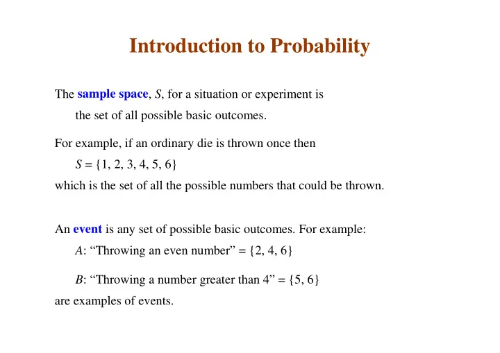
Introduction to Probability The sample space , S , for a situation or experiment is the set of all possible basic outcomes. For example, if an ordinary die is thrown once then S = {1, 2, 3, 4, 5, 6} which is the set of all the possible numbers
Introduction to Probability The sample space , S , for a situation or experiment is the set of all possible basic outcomes. For example, if an ordinary die is thrown once then S = {1, 2, 3, 4, 5, 6} which is the set of all the possible numbers that could be thrown. An event is any set of possible basic outcomes. For example: A : “Throwing an even number” = {2, 4, 6} B : “Throwing a number greater than 4” = {5, 6} are examples of events.
A set of events is mutually exclusive if no two can occur at the same time. For example, {1, 3}, {2, 4} and {6} are three mutually exclusive events. A set of events is exhaustive if at least one of them is bound to occur. For example, {1, 2, 3}, {3, 4, 5} and {5, 6} are three exhaustive events.
The probability P( E ) of an event E is an indication of how likely that event is to happen. Probabilities have the following properties: • For any event E : 0 ≤ P( E ) ≤ 1 . • If an event is impossible then its probability is 0 . • If an event is certain then its probability is 1 . • If A and B are mutually exclusive events then: P( A or B ) = P( A ) + P( B ) (where “ A or B ” is the event that one or the other, or both occur). • The sum of the probabilities of a mutually exclusive and exhaustive set of events is 1 .
If A and B are events, then the event “ A and B ” (that both occur) is called the joint event . The conditional probability of event A , given that event B occurs, P( A | B ) , is defined by: P( and ) A B = P( | ) A B P( ) B It follows that the joint probability = × P( and ) P( | ) P( ) A B A B B If A is any event and { E1 , E2 , … , En } are mutually exclusive and exhaustive events, then we have the generalized addition law : = + + + ! P( ) P( and 1) P( and 2) P( and ) A A E A E A En = × + × + + × ! P( ) P( | 1) P( 1) P( | 2) P( 2) P( | ) P( ) A A E E A E E A En En
Two events are said to be independent if the occurrence of one has no effect on the probability of the occurrence of the other. If events A and B are independent, then: = P( | ) P( ) A B A and so = × P( and ) P( ) P( ) A B A B
Three are three alternative interpretations of probability: Classical (or theoretical) probability: Based on simple games of chance involving symmetric objects such as fair coins, dice and packs of cards, in which basic outcomes are equally likely. For example, for a fair die: P(1) = P(2) = … = P(6) = 1/6 . In such simple cases, with finite sample spaces (i.e., with a finite number of basic outcomes), the probability of an event E is simply: number of basic outcomes in E E = P( ) number of basic outcomes in sample space For example, if E is the event of throwing a number greater than 4 with a fair die, then P( E ) = 2/6 = 1/3 .
Long-term frequency : Based on observing n repeated trials of an experiment and counting the number of times m that a particular event E occurs. The relative frequency, m / n , with which the event occurs is an estimate of the probability of E . As n is increased, this ratio becomes a more and more accurate estimate of the probability. m = ( ) P E Lim n →∞ n This interpretation applies to a far wider range of phenomena than does classical probability, for example to industrial processes and to life insurance.
Subjective probability: A measure of the degree of belief one has that an event will occur. It is a personal judgment, based on all relevant information one has at the time, such as a bookie’s odds in a horse race. This interpretation is applicable to the widest range of phenomena as it neither requires symmetry (as in classical probability) nor repeatability of identical trials (as in the frequentist approach). It is the most appropriate interpretation in the area of management decision making.
Bayes’ Theorem If A and B are any two events then: = × P( and ) P( | ) P( ) A B A B B Similarly: = × P( and ) P( | ) P( ) B A B A A But the joint event “ A and B” is the same as “ B and A” and so we can equate the probabilities. Therefore: × = × P( | ) P( ) P( | ) P( ) A B B B A A P( | ) B A = × and so: P( | ) P( ) A B A P( ) B Bayes’ theorem can be seen as relating P( A | B ) , the conditional probability of A given B , to the absolute probability P( A ).
If { A1 , A2 , … , An } are mutually exclusive and exhaustive, then for any one of the Ai : × P( | ) P( ) B Ai Ai = P( | ) Ai B × + + × ! P( | 1 ) P( 1 ) P( | ) P( ) B A A B An An We often use Bayes’ Theorem when we want to find the probability of a particular state of affairs, in the light of observations or experiments that have been made. If A1 , A2 , … , An are alternative states and observation B has been made, the last equation shows how to relate: the conditional probability that state Ai is the true state, given observation B to the “absolute” probability of Ai , estimated before B had been observed. Bayes’ Theorem provides the mechanism for updating our estimate as to the chance of Ai being the true state, in the light of new information.
P( Ai ) is sometimes called the prior probability of Ai prior to collecting any extra relevant information or making any extra observations related to the possible occurrence of Ai . P( Ai | B ) is sometimes called the posterior probability of Ai posterior (i.e., after) observing that B occurred. P( B | Ai ) is sometimes called the likelihood of B the probability of observing B , in state Ai .
Example : Two opaque jars A and B each contain ten balls. Jar A contains four red balls and six green balls. Jar B contains eight red balls and two green balls. A B One of the two jars is chosen at random. What is the probability that jar A was chosen?
In the absence of any further information, the Laplace criterion gives us the answer 1/2. i.e., the prior probability is: P( A ) = 1/2. Now suppose that some information is collected to help in deciding which jar was chosen. A ball is taken at random from the jar. It turns out to be a red ball. What effect does this have on the assessment of the probability that jar A had been chosen?
If jar A had been chosen, the probability that a red ball would be withdrawn is 4/10. If jar B had been chosen, the probability that a red ball would be withdrawn is 8/10. The likelihoods of a red ball being withdrawn are: P( red | A ) = 4/10, P( red | B ) = 8/10.
But we are interested in the posterior probability P( A | red ) . Using Bayes’ Theorem: × P( | ) P( ) red A A = P( | ) A red × + × P( | ) P( ) P( | ) P( ) red A A red B B × 4 / 10 1 / 2 = × + × ( 4 / 10 1 / 2 ) ( 8 / 10 1 / 2 ) 1 / 5 = + 1 / 5 2 / 5 = 1 / 3
It is sometimes easier to employ a diagrammatic method based on Bayes’ theorem, which involves: !" drawing a unit square, !" marking the a priori probabilities along the base, !" dividing the square into corresponding vertical rectangles, !" dividing each rectangle according to the likelihood values, and !" calculating the area of each of the resulting smaller rectangles. 0.1 0.2 = P( green | B ) P( green | A ) = 0.6 0.3 0.4 0.8 = P( red | B ) P( red | A ) = 0.4 0.2 0.5 0.5 = P( A ) = P( B )
The two original vertical rectangles correspond to the two events: “jar A was picked” and “jar B was picked”. Each of the smaller rectangles represents a joint event, such as “jar A was picked and a red ball was drawn from it”. The areas of the rectangles are the probabilities of these different events. 0.1 0.2 = P( green | B ) P( green | A ) = 0.6 0.3 0.4 0.8 = P( red | B ) P( red | A ) = 0.4 0.2 0.5 0.5 = P( A ) = P( B )
The rectangles shaded red represent the two joint events which involve drawing a red ball. The overall probability of such a result is: P( red ) = P( A and red ) + P( B and red ) = P( red | A ) x P( A ) + P( red | B ) x P ( B ) = 0.4 x 0.5 + 0.8 x 0.5 = 0.2 + 0.4 = 0.6 The regions shaded green represent the joint events that involve drawing a green ball: P( green ) = P( A and green ) + P( B and green ) = P( green | A ) x P( A ) + P( green | B ) x P( B ) = 0.6 x 0.5 + 0.2 x 0.5 = 0.3 + 0.1 = 0.4
The posterior probabilities are: × P( | ) P( ) red A A P( and ) A red 0 . 2 P( A | red ) = = = = 1/3 P( ) P( ) red red 0 . 6 × P( | ) P( ) red B B P( and ) B red 0 . 4 P( B | red ) = = = = 2/3 P( ) P( ) red red 0 . 6 × P( | ) P( ) green A A P( and ) 0 . 3 A green P( A | green ) = = = = 3/4 P( ) P( ) green green 0 . 4 × 0 . 1 P( and ) P( | ) P( ) B green green B B P( B | green ) = = = = 1/4 0 . 4 P( ) P( ) green green
Drawing a red ball : decreases the probability of jar A from 1/2 to 1/3 and increases the probability of jar B from 1/2 to 2/3. Drawing a green ball : increases the probability of jar A from 1/2 to 3/4 and decreases the probability of jar B from 1/2 to 1/4.
Recommend
More recommend
Explore More Topics
Stay informed with curated content and fresh updates.
