Chapter 5. Continuous-Time Markov Chains Prof. Shun-Ren Yang - PowerPoint PPT Presentation
Chapter 5. Continuous-Time Markov Chains Prof. Shun-Ren Yang Department of Computer Science, National Tsing Hua University, Taiwan Continuous-Time Markov Chains Consider a continuous-time stochastic process { X ( t ) , t 0 } taking on
Chapter 5. Continuous-Time Markov Chains Prof. Shun-Ren Yang Department of Computer Science, National Tsing Hua University, Taiwan
Continuous-Time Markov Chains • Consider a continuous-time stochastic process { X ( t ) , t ≥ 0 } taking on values in the set of nonnegative integers. We say that the process { X ( t ) , t ≥ 0 } is a continuous-time Markov chain if for all s, t ≥ 0, and nonnegative integers i, j, x ( u ) , 0 ≤ u ≤ s , P { X ( t + s ) = j | X ( s ) = i, X ( u ) = x ( u ) , 0 ≤ u < s } = P { X ( t + s ) = j | X ( s ) = i } . • In other words, a continuous-time Markov chain is a stochastic process having the Markovian property that the conditional distribution of the future state at time t + s , given the present state at s and all past states depends only on the present state and is independent of the past. • Suppose that a continuous-time Markov chain enters state i at some time, say time 0, and suppose that the process does not leave state i Prof. Shun-Ren Yang, CS, NTHU 1
Continuous-Time Markov Chains (that is, a transition does not occur) during the next s time units. What is the probability that the process will not leave state i during the following t time units? • Note that as the process is in state i at time s , it follows, by the Markovian property, that the probability it remains in that state during the interval [ s, s + t ] is just the (unconditional) probability that it stays in state i for at least t time units. That is, if we let τ i denote the amount of time that the process stays in state i before making a transition into a different state, then P { τ i > s + t | τ i > s } = P { τ i > t } for all s, t ≥ 0. Hence, the random variable τ i is memoryless and must thus be exponentially distributed. Prof. Shun-Ren Yang, CS, NTHU 2
Continuous-Time Markov Chains • In fact, the above gives us a way of constructing a continuous-time Markov chain. Namely, it is a stochastic process having the properties that each time it enters state i : 1. the amount of time it spends in that state before making a transition into a different state is exponentially distributed with rate, say, v i ; and 2. when the process leaves state i , it will next enter state j with some probability, call it P ij , where � j � = i P ij = 1. • A state i for which v i = ∞ is called an instantaneous state since when entered it is instantaneously left. If v i = 0, then state i is called absorbing since once entered it is never left. • Hence, a continuous-time Markov chain is a stochastic process that moves from state to state in accordance with a (discrete-time) Markov Prof. Shun-Ren Yang, CS, NTHU 3
Continuous-Time Markov Chains chain, but is such that the amount of time it spends in each state, before proceeding to the next state, is exponentially distributed. • In addition, the amount of time the process spends in state i , and the next state visited, must be independent random variables. For if the next state visited were dependent on τ i , then information as to how long the process has already been in state i would be relevant to the prediction of the next state — and this would contradict the Markovian assumption. • Let q ij be defined by q ij = v i P ij , all i � = j. Since v i is the rate at which the process leaves state i and P ij is the probability that it then goes to j , it follows that q ij is the rate when in state i that the process makes a transition into state j ; and in fact we Prof. Shun-Ren Yang, CS, NTHU 4
Continuous-Time Markov Chains call q ij the transition rate from i to j . • Let us denote by P ij ( t ) the probability that a Markov chain, presently in state i , will be in state j after an additional time t . That is, P ij ( t ) = P { X ( t + s ) = j | X ( s ) = i } . Prof. Shun-Ren Yang, CS, NTHU 5
Birth and Death Processes • A continuous-time Markov chain with states 0 , 1 , . . . for which q ij = 0 whenever | i − j | > 1 is called a birth and death process . • Thus a birth and death process is a continuous-time Markov chain with states 0 , 1 , . . . for which transitions from state i can only go to either state i − 1 or state i + 1. The state of the process is usually thought of as representing the size of some population, and when the state increases by 1 we say that a birth occurs, and when it decreases by 1 we say that a death occurs. • Let λ i and µ i be given by λ i = q i,i +1 , µ i = q i,i − 1 . The values { λ i , i ≥ 0 } and { µ i , i ≥ 1 } are called respectively the birth rates and the death rates. Prof. Shun-Ren Yang, CS, NTHU 6
Birth and Death Processes • Since � j q ij = v i , we see that v i = λ i + µ i , λ i P i,i +1 = = 1 − P i,i − 1 . λ i + µ i • Hence, we can think of a birth and death process by supposing that whenever there are i people in the system the time until the next birth is exponential with rate λ i and is independent of the time until the next death, which is exponential with rate µ i . Prof. Shun-Ren Yang, CS, NTHU 7
An Example: The M/M/s Queue • Suppose that customers arrive at an s-server service station in accordance with a Poisson process having rate λ . • Each customer, upon arrival, goes directly into service if any of the servers are free, and if not, then the customer joins the queue (that is, he waits in line). • When a server finishes serving a customer, the customer leaves the system, and the next customer in line, if there are any waiting, enters the service. The successive service times are assumed to be independent exponential random variables having mean 1 /µ . • If we let X ( t ) denote the number in the system at time t , then Prof. Shun-Ren Yang, CS, NTHU 8
An Example: The M/M/s Queue { X ( t ) , t ≥ 0 } is a birth and death process with ⎧ nµ 1 ≤ n ≤ s ⎨ µ n = sµ n > s, ⎩ λ n = λ, n ≥ 0 . Prof. Shun-Ren Yang, CS, NTHU 9
The Kolmogorov Differential Equations • Recall that P ij ( t ) = P { X ( t + s ) = j | X ( s ) = i } represents the probability that a process presently in state i will be in state j a time t later. • By exploiting the Markovian property, we will derive two sets of differential equations for P ij ( t ), which may sometimes be explicitly solved. However, before doing so we need the following lemmas. • Lemma 1. 1 − P ii ( t ) 1. lim = v i . t t → 0 P ij ( t ) 2. lim = q ij , i � = j . t t → 0 Prof. Shun-Ren Yang, CS, NTHU 10
The Kolmogorov Differential Equations • Lemma 2. For all s, t, ∞ � P ij ( t + s ) = P ik ( t ) P kj ( s ) . k =0 • From Lemma 2 we obtain � P ij ( t + h ) = P ik ( h ) P kj ( t ) , k or, equivalently, � P ij ( t + h ) − P ij ( t ) = P ik ( h ) P kj ( t ) − [1 − P ii ( h )] P ij ( t ) . k � = i Dividing by h and then taking the limit as h → 0 yields, upon Prof. Shun-Ren Yang, CS, NTHU 11
The Kolmogorov Differential Equations application of Lemma 1, P ij ( t + h ) − P ij ( t ) P ik ( h ) � lim = lim P kj ( t ) − v i P ij ( t ) . h h h → 0 h → 0 k � = i • Assuming that we can interchange the limit and summation on the right-hand side of the above equation, we thus obtain, again using Lemma 1, the following. • Theorem. (Kolmogorov’s Backward Equations) For all i, j, and t ≥ 0, P ′ � ij ( t ) = q ik P kj ( t ) − v i P ij ( t ) . k � = i Prof. Shun-Ren Yang, CS, NTHU 12
The Kolmogorov Differential Equations • The set of differential equations for P ij ( t ) given in the above Theorem are known as the Kolmogorov backward equations . • They are called the backward equations because in computing the probability distribution of the state at time t + h we conditioned on the state (all the way) back at time h . That is, we started our calculation with � P ij ( t + h ) = P { X ( t + h ) = j | X (0) = i, X ( h ) = k } k × P { X ( h ) = k | X (0) = i } � = P kj ( t ) P ik ( h ) . k Prof. Shun-Ren Yang, CS, NTHU 13
The Kolmogorov Differential Equations • We may derive another set of equations, known as the Kolmogorov’s forward equations , by now conditioning on the state at time t . This yields � P ij ( t + h ) = P ik ( t ) P kj ( h ) k or � P ij ( t + h ) − P ij ( t ) = P ik ( t ) P kj ( h ) − P ij ( t ) k � = P ik ( t ) P kj ( h ) − [1 − P jj ( h )] P ij ( t ) . k � = j Therefore, P ik ( t ) P kj ( h ) P ij ( t + h ) − P ij ( t ) − 1 − P jj ( h ) � lim = lim h → 0 { P ij ( t ) } . h h h h → 0 k � = j Prof. Shun-Ren Yang, CS, NTHU 14
The Kolmogorov Differential Equations • Assuming that we can interchange limit with summation, we obtain by Lemma 1 that P ′ � ij ( t ) = q kj P ik ( t ) − v j P ij ( t ) . k � = j • Theorem. (Kolmogorov’s Forward Equations) Under suitable regularity conditions, P ′ � ij ( t ) = q kj P ik ( t ) − v j P ij ( t ) . k � = j Prof. Shun-Ren Yang, CS, NTHU 15
The Kolmogorov Differential Equations Example. The Two-State Chain. Consider a two-state continuous-time Markov chain that spends an exponential time with rate λ in state 0 before going to state 1, where it spends an exponential time with rate µ before returning to state 0. The forward equations yield P ′ 00 ( t ) = µP 01 ( t ) − λP 00 ( t ) = − ( λ + µ ) P 00 ( t ) + µ, where the last equation follows from P 01 ( t ) = 1 − P 00 ( t ). Hence, e ( λ + µ ) t [ P ′ 00 ( t ) + ( λ + µ ) P 00 ( t )] = µe ( λ + µ ) t or d dt [ e ( λ + µ ) t P 00 ( t )] = µe ( λ + µ ) t . Prof. Shun-Ren Yang, CS, NTHU 16
Recommend
More recommend
Explore More Topics
Stay informed with curated content and fresh updates.
