Bayesian Methods for Parameter Estimation Bayesian vs Frequentist - PowerPoint PPT Presentation

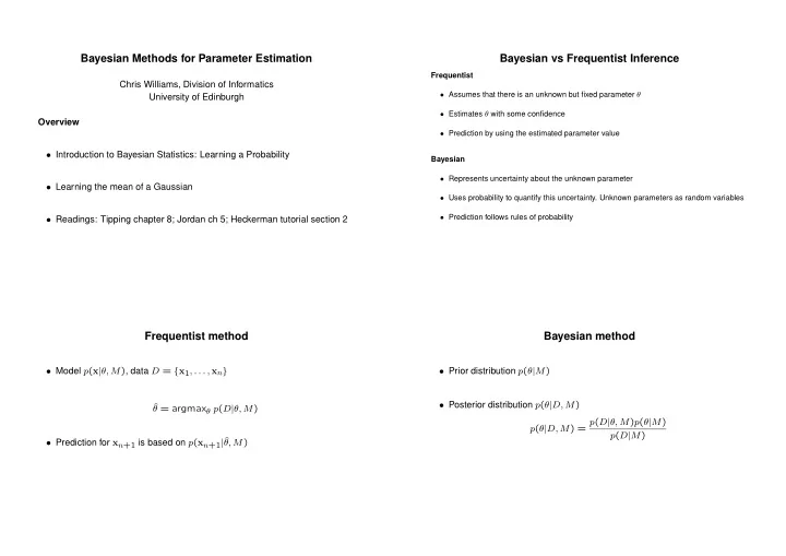
Bayesian Methods for Parameter Estimation Bayesian vs Frequentist Inference Frequentist Chris Williams, Division of Informatics • Assumes that there is an unknown but fixed parameter θ University of Edinburgh • Estimates θ with some confidence Overview • Prediction by using the estimated parameter value • Introduction to Bayesian Statistics: Learning a Probability Bayesian • Represents uncertainty about the unknown parameter • Learning the mean of a Gaussian • Uses probability to quantify this uncertainty. Unknown parameters as random variables • Prediction follows rules of probability • Readings: Tipping chapter 8; Jordan ch 5; Heckerman tutorial section 2 Frequentist method Bayesian method • Model p ( x | θ, M ) , data D = { x 1 , . . . , x n } • Prior distribution p ( θ | M ) • Posterior distribution p ( θ | D, M ) ˆ θ = argmax θ p ( D | θ, M ) p ( θ | D, M ) = p ( D | θ, M ) p ( θ | M ) p ( D | M ) • Prediction for x n +1 is based on p ( x n +1 | ˆ θ, M )

Bayes, MAP and Maximum Likelihood • Making predictions � p ( x n +1 | D, M ) = p ( x n +1 , θ | D, M ) dθ � p ( x n +1 | D, M ) = p ( x n +1 | θ, M ) p ( θ | D, M ) dθ � = p ( x n +1 | θ, D, M ) p ( θ | D, M ) dθ • Maximum a posteriori value of θ θ MAP = argmax θ p ( θ | D, M ) � = p ( x n +1 | θ, M ) p ( θ | D, M ) dθ Note: not invariant to reparameterization (cf ML estimator) Interpretation: average of predictions p ( x n +1 | θ, M ) weighted by • If posterior is sharply peaked about the most probable value θ MAP then p ( θ | D, M ) p ( x n +1 | D, M ) ≃ p ( x n +1 | θ MAP , M ) • In the limit n → ∞ , θ MAP converges to ˆ θ (as long as p (ˆ θ ) � = 0 ) • Marginal likelihood (important for model comparison) • Bayesian approach most effective when data is limited, n is small � p ( D | M ) = P ( D | θ, M ) P ( θ | M ) dθ Learning probabilities: thumbtack example Likelihood Frequentist Approach • Likelihood for a sequence of heads and tails • The probability of heads θ is un- heads tails known p ( hhth . . . tth | θ ) = θ n h (1 − θ ) n t • Given iid data, estimate θ using an estimator with good proper- • MLE ties (e.g. ML estimator) n h ˆ θ = n h + n t

Learning probabilities: thumbtack example Examples of the Beta distribution 3.5 2 Bayesian Approach: (a) the prior 1.8 3 1.6 1.4 2.5 1.2 2 1 0.8 1.5 0.6 • Prior density p ( θ ) , use beta distribution 0.4 1 0.2 0.5 0 0 0.1 0.2 0.3 0.4 0.5 0.6 0.7 0.8 0.9 1 0 0.1 0.2 0.3 0.4 0.5 0.6 0.7 0.8 0.9 1 p ( θ ) = Beta( α h , α t ) ∝ θ α h − 1 (1 − θ ) α t − 1 Beta(0.5,0.5) Beta(1,1) 1.8 4.5 for α h , α t > 0 1.6 4 1.4 3.5 1.2 3 1 2.5 0.8 2 0.6 1.5 0.4 1 • Properties of the beta distribution 0.2 0.5 0 0 0 0.1 0.2 0.3 0.4 0.5 0.6 0.7 0.8 0.9 1 0 0.1 0.2 0.3 0.4 0.5 0.6 0.7 0.8 0.9 1 α h � E [ θ ] = θp ( θ ) = α h + α t Beta(3,2) Beta(15,10) Bayesian Approach: (b) the posterior Bayesian Approach: (c) making predictions p ( θ | D ) ∝ p ( θ ) p ( D | θ ) θ ∝ θ α h − 1 (1 − θ ) α t − 1 θ n h (1 − θ ) n t ∝ θ α h + n h − 1 (1 − θ ) α t + n t − 1 x x x x n+1 n 1 2 • Posterior is also a Beta distribution ∼ Beta( α h + n h , α t + n t ) • The Beta prior is conjugate to the binomial likelihood (i.e. they have the � p ( X n +1 = heads | D, M ) = p ( X n +1 = heads | θ ) p ( θ | D, M ) dθ same parametric form) � = θ Beta(( α h + n h , α t + n t ) dθ • α h and α t can be thought of as imaginary counts, with α = α h + α t as the equivalent sample size = α h + n h α + n

Beyond Conjugate Priors • The thumbtack came from a magic shop → a mixture prior p ( θ ) = 0 . 4Beta(20 , 0 . 5) + 0 . 2Beta(2 , 2) + 0 . 4Beta(0 . 5 , 20) Generalization to multinomial variables • Posterior distribution r � • Dirichlet prior θ α i + n i − 1 p ( θ | n 1 , . . . , n r ) ∝ i r i =1 � θ α i − 1 p ( θ 1 , . . . , θ r ) = Dir( α 1 , . . . , α r ) ∝ i • Marginal likelihood i =1 with r Γ( α ) Γ( α i + n i ) � p ( D | M ) = � θ i = 1 , α i > 0 Γ( α + n ) Γ( α i ) i =1 i • α i ’s are imaginary counts, α = � i α i is equivalent sample size • Properties E ( θ i ) = α i α • Dirichlet distribution is conjugate to the multinomial likelihood

Inferring the mean of a Gaussian with n x = 1 � x i n i =1 • Likelihood nσ 2 σ 2 p ( x | µ ) ∼ N ( µ, σ 2 ) 0 µ n = 0 + σ 2 x + 0 + σ 2 µ 0 nσ 2 nσ 2 1 σ 2 + 1 = n • Prior σ 2 σ 2 p ( µ ) ∼ N ( µ 0 , σ 2 n 0 0 ) • See Tipping § 8.3.1 for details • Given data D = { x 1 , . . . , x n } , what is p ( µ | D ) ? p ( µ | D ) ∼ N ( µ n , σ 2 n ) Comparing Bayesian and Frequentist approaches • Frequentist : fi x θ , consider all possible data sets generated with θ fi xed • Bayesian : fi x D , consider all possible values of θ • One view is that Bayesian and Frequentist approaches have different defi nitions of what it means to be a good estimator