10/16/19 Parameter Control Genetic Algorithms Motivation - PDF document
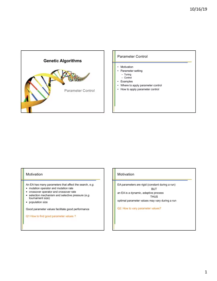
10/16/19 Parameter Control Genetic Algorithms Motivation Parameter setting Tuning Control Examples Where to apply parameter control How to apply parameter control Parameter Control Motivation Motivation An EA
10/16/19 Parameter Control Genetic Algorithms • Motivation • Parameter setting – Tuning – Control • Examples • Where to apply parameter control • How to apply parameter control Parameter Control Motivation Motivation An EA has many parameters that affect the search, e.g. EA parameters are rigid (constant during a run) mutation operator and mutation rate BUT crossover operator and crossover rate an EA is a dynamic, adaptive process selection mechanism and selective pressure ( e.g. THUS tournament size) optimal parameter values may vary during a run population size Q2: How to vary parameter values? Good parameter values facilitate good performance Q1 How to find good parameter values ? 1
10/16/19 Parameter Settings: Parameter Setting Tuning Parameter tuning: the traditional way of testing and comparing different values before the “real” run Problems: users mistakes in settings can be sources of errors or sub-optimal performance parameters interact: exhaustive search is not practicable costs much time even with “smart” tuning good values may become bad during the run Parameter Settings: Examples: Control Varying mutation step size Parameter control: setting values on-line, during the Problem to solve: actual run, e.g. min f(x 1 ,…,x n ) L i £ x i £ U i predetermined time-varying schedule p = p(t) for i = 1,…,n bounds finding optimal p is hard, finding optimal p(t) is harder g j (x) £ 0 for j = 1,…,q inequality constraints h k (x) = 0 for k = q+1,…,m equality constraints using feedback from the search process still user-defined feedback mechanism, how to ``optimize"? Algorithm: EA with real-valued representation x = (x 1 ,…,x n ) encoding parameters in chromosomes and rely on arithmetic averaging crossover selection Gaussian mutation: x’ i = x i + N(0, s ) will natural selection work for strategy parameters? standard deviation s is called mutation step size how to implement effectively? 2
10/16/19 Examples: Examples: Varying mutation step size, option 1 Varying mutation step size, option 2 Replace the constant s by a function s (t) Replace the constant s by a function s (t) updated after every n steps by the 1/5 success rule: σ ( t )= 1 - 0 .9 × t T 0 £ t £ T is the current generation number 1/5 success rule (Rechenberg 1973): 1/5 of mutations should be successful – mutant more fit Characteristics: than parent changes in s are independent from the search progress strong user control of s by the above formula s is fully predictable a given s acts on all individuals of the population Examples: Examples: Varying mutation step size, option 2 Varying mutation step size, option 3 Replace the constant s by a function s (t) updated after Assign a personal s to each individual every n steps by the 1/5 success rule: Incorporate this s into the chromosome: (x 1 , …, x n , s ) Apply variation operators to x i ‘s and s ì s (t - n) / c if p > 0 . 2 σ ' = σ × e N( 0, σ ) s ï s s - × < (t) = (t n) c if p 0 . 2 0 < # < 1 í s x i ' = x i +N( 0, σ ' ) ï s - (t n) otherwise î Characteristics: Characteristics: changes in s are results of natural selection changes in s are based on feedback from the search progress (almost) no user control of s some user control of s by the above formula s is not predictable s is not predictable a given s acts on one individual a given s acts on all individuals of the population 3
10/16/19 Examples: Examples: Varying mutation step size, option 4 Varying penalties Constraints Assign a personal s to each variable in each individual Incorporate s ’s into the chromosomes: (x 1 , …, x n , s 1 , …, s n ) g j (x) £ 0 for j = 1,…,q inequality constraints h k (x) = 0 for k = q+1,…,m equality constraints Apply variation operators to x i ‘s and s i ‘s are handled by penalties: σ i ' = σ i × e N( 0, τ ) x i ' = x i +N( 0, σ i ' ) eval(x) = f(x) + W × penalty(x) Characteristics: changes in s i are results of natural selection where (almost) no user control of s i ì 1 for violated constrai nt m s i is not predictable å = penalty ( x ) í a given s i acts on one gene of one individual 0 for satisfied constrai nt = î j 1 Examples: Examples: Varying penalties, option 1 Varying penalties, option 2 Replace the constant W by a function W(t) Replace the constant W by W(t) updated in each generation b ´ ì W(t) if last k champions all feasible ´ α W(t) = ( C t) ï g ´ W(t + 1 ) = í W(t) if last k champions all infeasible ï W(t) otherwise 0 £ t £ T is the current generation number î b < 1, g > 1, b ´ g ¹ 1 champion: best of its generation Characteristics: changes in W independent from the search progress Characteristics: strong user control of W by the above formula changes in W are based on feedback from the search progress some user control of W by the above formula W is fully predictable W is not predictable a given W acts on all individuals of the population a given W acts on all individuals of the population 4
10/16/19 Examples: Examples: Varying penalties, option 3 Lessons learned Assign a personal W to each individual in population Various forms of parameter control can be distinguished by: Incorporate this W into the chromosome: (x 1 , …, x n , W) Apply variation operators to W and each x i primary features: what component of the EA is changed Alert: how the change is made eval ((x, W)) = f (x) + W × penalty(x) secondary features: while for mutation step sizes we had evidence/data backing up changes eval ((x, s )) = f (x) level/scope of change this option is thus “cheating” Þ algorithm can improve the evaluation by evolving smaller weights W rather than improving f(x) Examples: Where to apply parameter control Lessons learned Various forms of parameter control can be distinguished by: Practically any EA component can be parameterized and thus controlled on-the-fly: representation (x 1 , ..., x n , σ) (x 1 , …, x n , σ 1 , (x 1 , ..., x n , W) σ(t) = 1-0.9*t/T σ' = σ/c, if r > W(t) = (C*t) α W'= β *W, if b i ∈ F ⅕ ... …, σ n ) evaluation function What Step size Step size Step Step Penalty Penalty Penalty variation operators size size weight weight weight selection operator (parent or mating selection) How Deterministic Adaptive Self- Self- Deterministic Adaptive Self- adaptive adaptive adaptive replacement operator (survival or environmental Time (Fitness) (Fitness) Time Constraint (Fitness) Evidence Successful selection) mutations satisfaction rate history population (size, topology) Scope Population Population Individual Gene Population Population Individual 5
10/16/19 How to apply parameter control How to apply parameter control Global taxonomy Three major types of parameter control: deterministic: some rule modifies strategy parameter without feedback from the search (based on some counter) adaptive: feedback rule based on some measure monitoring search progress self-adaptative: parameter values evolve along with solutions; encoded onto chromosomes they undergo variation and selection Evidence: Evidence: Informing the change Informing the change The parameter changes may be based on: Absolute evidence: predefined event triggers change, e.g. increase p m by 10% if population diversity falls under time or nr. of evaluations (deterministic control) threshold x population statistics (adaptive control) Direction and magnitude of change is fixed progress made population diversity Relative evidence: compare values through solutions gene distribution, etc. created with them, e.g. increase p m if top quality offspring came by high mutation rates relative fitness of individuals created with given values Direction and magnitude of change is not fixed (adaptive or self-adaptive control) 6
10/16/19 Evidence: Scope/level Refined taxonomy The parameter may take effect on different levels: l Combinations of types and evidences l Possible: + environment (fitness function) l Impossible: - population individual sub-individual Note: given component (parameter) determines possibilities Thus: scope/level is a derived or secondary feature in the classification scheme Evaluation/Summary Parameter control offers the possibility to use appropriate values in various stages of the search Adaptive and self-adaptive parameter control offer users “liberation” from parameter tuning delegate parameter setting task to the evolutionary process the latter implies a double task for an EA: problem solving + self- calibrating (overhead) 7
Recommend
More recommend
Explore More Topics
Stay informed with curated content and fresh updates.
