A Frequentist Semantics for a Generalized Jeffrey Conditionalization - PowerPoint PPT Presentation
A Frequentist Semantics for a Generalized Jeffrey Conditionalization Dirk Draheim Tallinn University of Technology, 5th May 2016 Motivation Partial knowledge specification Probability conditional on list of frequency castings
A Frequentist Semantics for a Generalized Jeffrey Conditionalization Dirk Draheim Tallinn University of Technology, 5th May 2016
Motivation • Partial knowledge specification • Probability conditional on list of frequency castings • Bayesian epistemology vs. classical, frequentist extensio of probability theory P ( A | B 1 ≡ b 1 , . . . , B n ≡ b n ) (1) P ( A | B ≡ b ) (2) 1
Many-Valued Logics L δ Gödel logics Gk Lukasiewicz Product logic Post logics logics Lk Π Pm A ∧ B ≤ min {A,B} min{A,B} 1-min{1,1-A-B} ¬ A 1-A 1, if A=0 1-A 1, A=0 0, if A>0 A-(1/(m-1)), A>0 A ∨ B ≥ max {A,B} max{A,B} min{1,A+B} max{A,B} A → B ≤ min {1-A,B} 1, if A ≤ B min{1,1-A+B} B, if A>B 2
Jeffrey Conditionalization Conditional Proabability P ( A | B ) = P ( AB ) (3) P ( B ) Jeffrey Conditionalization – Probability Kynematics P ( A | B ≡ b ) = b · P ( A | B ) + (1 − b ) · P ( A | B ) (4) Conditional Proabality as Jeffrey Conditionalization P ( A | B ) = P ( A | B ≡ 100%) (5) P ( A | B ) = P ( A | B ≡ 0%) (6) 3
Frequentist Semantics of Jeffrey Conditionalization We define: P n ( A | B ≡ b ) = DEF E ( A n | B n = b ) (7) We have: P n ( A | B ≡ b ) = P ( A | B n = b ) (8) Lemma 1 ( Bounded F.P. Conditionalization in the Basic Jeffrey Case) Let b = x/y so that x/y is the irreducable fraction of b . For all n = m · y with m ∈ N we have the following: P n ( A | B ≡ b ) = b · P ( A | B ) + (1 − b ) · P ( A | B ) (9) In particular: P 1 ( A | B ≡ 100%) = P ( A | B 1 = 1) = P ( A | B ) (10) 4
Frequentist Semantics of F.P. Conditionalization Given b = b 1 , . . . , b n so that y is the least common denominator of b . For all n = m · y with m ∈ N we define bounded F.P. conditionalization: P n ( A | B 1 ≡ b 1 , . . . , B n ≡ b n ) = DEF E ( A n | B 1 n = b 1 . . . , B m n ) (11) We have: P n ( A | B 1 ≡ b 1 , . . . , B n ≡ b n ) = DEF P ( A | B 1 n = b 1 . . . , B m n ) (12) P n ( A | B ≡ b ) = DEF P ( A | B n = b ) (13) We define F.P. conditionalization: where n = n ′ · lcd ( b ) n ′ →∞ P n ( A | B ≡ b ) P ( A | B ≡ b ) = lim (14) 5
Proof of Lemma 1 P n ( A | B ≡ b ) (15) P ( A | B n = b ) (16) P ( A, B n = b ) (17) P ( B n = b ) P ( AB, B n = b ) + P ( AB, B n = b ) (18) P ( B n = b ) P ( B n = b ) We consider the first summand only: P ( AB, B n = b ) (19) P ( B n = b ) 6
Proof of Lemma 1 – cont. (ii) P ( A 1 B 1 , B 1 + · · · + B n = b ) (20) P ( B n = b ) P ( A 1 B 1 , B 2 + · · · + B n = bn − 1 n − 1 ) (21) P ( B n = b ) P ( A 1 B 1 ) · P ( B 2 + · · · + B n = bn − 1 n − 1 ) (22) P ( B n = b ) Now, due to the fact that ( B i ) i ∈ N is a sequence of i.i.d random variables, we have the following: P ( B 2 + · · · + B n = bn − 1 1 ) = bn − 1 n − 1 ) = P ( B 1 + · · · + B n (23) − n − 1 Due to Eqn. (23) we can rewrite Eqn. (22), just for convenience and better readability, as follows: P ( AB ) · P ( B n − 1 = bn − 1 n − 1 ) (24) P ( B n = b ) 7
Proof of Lemma 1 – cont. (iii) Now, we have that P ( AB ) equals P ( A | B ) · P ( B ) and therefore that Eqn. (24) equals: P ( A | B ) · P ( B ) · P ( B n − 1 = bn − 1 n − 1 ) (25) P ( B n = b ) As the next crucial step, we resolve P ( B n − 1 = bn − 1 n − 1 ) and P ( B n = b ) combinatorically. We have that Eqn. (25) equals: � n − 1 · P ( B ) bn − 1 · P ( B ) n − bn � bn − 1 P ( A | B ) · P ( B ) · � n (26) � · P ( B ) bn · P ( B ) n − bn bn As a next step, we can cancel all occurrences of P ( B ) and P ( B ) from Eqn. (26) which yields the following: ( n − 1)! n ! � P ( A | B ) · (27) ( bn − 1)!( n − 1 − ( bn − 1))! ( bn )!( n − bn )! After resolving ( n − 1)! as n ! /n , resolving ( bn − 1)! to ( bn )! / ( bn ) and some further trivial transformations we have that Eqn. (27) equals: n ( bn )!( n − bn )! · ( bn )!( n − bn )! n ! bn P ( A | B ) · (28) n ! 8
Proof of Lemma 1 – cont. (iv) Now, after a series of further cancelations we have that Eqn. (28) equals the following: b · P n ( A | B ) (29) Similarly (omitted), it can be shown that the second summand in Eqn. (18) equals: (1 − b ) · P n ( A | B ) (30) � 9
Decomposition of F.P. Conditionalization Lemma 2 (Decomposition of Bounded F.P. Conditionalization) Given a bounded F.P. conditionalization P n ( A | B ≡ b ) for some bound n and a vector of events B = ( B i ) { 1 ,...,m } for the index set I = { 1 , . . . , m } , we have the following: � � P n ( A | B ≡ b ) = i ∈ I ζ i ) · P n ( ∩ � P ( A | ∩ i ∈ I ζ i | B ≡ b ) (31) � � ζ i ∈ { B i , B i } i ∈ I P ( ∩ i ∈ I ζ i ) � = 0 For example, in case of two conditions: P ( A | B ≡ b, C ≡ c ) = P ( A | BC ) · P ( BC | B ≡ b, C ≡ c ) + P ( A | BC ) · P ( BC | B ≡ b, C ≡ c ) (32) + P ( A | BC ) · P ( BC | B ≡ b, C ≡ c ) + P ( A | BC ) · P ( BC | B ≡ b, C ≡ c ) 10
Computation of F.P. Conditionalization Definition 3 (Frequency Adoption) np − 1 ⎧ , l ∈ J ξ l,n ⎨ n − 1 J ( p ) = (33) np , l �∈ J ⎩ n − 1 Based on the notation for frequency adoption in Def. 3, we can define the computation of F.P. conjunctions via the following recursive equation: P n ( B 1 ≡ b 1 . . . B m ≡ b m ) ⎧ 1 , n = 0 ⎪ ⎪ ⎪ ⎪ B 1 ≡ ξ 1 ,n I ′ ( b 1 ) ,.., B m ≡ ξ m,n ⎪ � � · P n − 1 � � ⎪ ( b m ) , n � 1 � P i ∈ I ′ B i , ∩ ∩ i ∈ I ′ B i (34) ⎪ I ′ ⎨ = I ′ ⊆ I ⎪ ⎪ ∄ i ∈ I ′ .b i =0 ⎪ ⎪ ⎪ ⎪ ∄ i ∈ I ′ .b i =1 ⎪ ⎩ 11
F.P. Conditionalization and Independency Lemma 4 (Independence of F.P. Conditions) Given a bounded F.P. conditionalization P n ( A | B ≡ b ) for some bound n and a vector of mutually independent events B = ( B i ) { 1 ,...,m } for the index set I = { 1 , . . . , m } , we have the following: � � P n ( A | B ≡ b ) = � � � P ( A | i ∈ I ′ B i , ∩ ∩ i ∈ I ′ B i ) · b i · (1 − b i ) (35) I ′ ⊆ I i ∈ I ′ i ∈ I ′ For example, in case of two conditions: P ( A | B ≡ b, C ≡ c ) = P ( A | BC ) · bc + P ( A | BC ) · b (1 − c ) (36) + P ( A | BC ) · (1 − b ) c + P ( A | BC ) · (1 − b )(1 − c ) 12
Outlook – Bayesianism and Frequentism • Jakob Bernoulli • Bruno de Finetti • John Maynard Keynes • Frank P. Ramsey • Rudolf Carnap • Dempster-Shafer 13
Conclusion • Partial knowledge specification • Probability conditional on list of frequency castings • Bayesian epistemology vs. classical, frequentist extensio of probability theory • P ( A | B 1 ≡ b 1 , . . . , B n ≡ b n ) • P ( A | B ≡ b ) • In its basic case, F.P. conditionalization meets Jeffrey conditionalization • Computation of F.P. conditionalization • Independency and F.P. conditionalization • F.P. conditionalization and Bayesianism vs. frequentism 14
Thanks a lot! dirk.draheim@ttu.ee 15
Appendix 16
Definition 5 (Independent Random Variables) Given to random variables X : Ω → I and Y : Ω → I , we say that and X and Y are independent, if the following holds for all v ∈ I and v ′ ∈ I : P ( X = v, Y = v ′ ) = P ( X = v ) · P ( Y = v ′ ) (37) Definition 6 (Identically Distributed Random Variables) Given to random variables X : Ω → I and Y : Ω → I , we say that and X and Y are identically distributed, if the following holds for all v ∈ I : P ( X = v ) = P ( Y = v ) (38) Definition 7 (Independent, Identically Distributed) Given to random variables X : Ω → I and Y : Ω → I , we say that and X and Y are independent identically distributed, abbreviated as i.i.d , if they are both independent and identically distributed. Definition 8 (Sequence of i.i.d Random Variables) Random variables ( X i ) i ∈ N are called independent identically distributed, again abbreviated as i.i.d , if they are pairwise independent and furthermore identically distributed. 17
Definition 9 (Matrix of i.i.d Random Variables) Given a list ( X k ) k ∈ R with R = { 1 , . . . , m } of sequences of random variables X k = ( X ki ) i ∈ N so that ( X ki ) : Ω − → I , i.e., random variables that are organized in an R × N -matrix. These random variables are called independent identically distributed, again abbreviated as i.i.d , if each row X k for all k ∈ R is identically distributed and furthermore, they are column-wise mutually completely independent as defined as follows. Given a designated column number c ∈ N , numbers 1 � n � m , 1 � n ′ � m , a sequence of row indices i 1 , . . . , i n , a sequence of row indices j 1 , . . . , j n ′ , and a sequence of column indices k 1 , . . . , k n ′ so that k q � = c for all 1 � q � n ′ we have that the following independency condition holds: P ( X i 1 c ,..., X i n c , X j 1 k 1 ,..., X j n ′ k n ′ ) = P ( X i 1 c ,..., X i n c ) · P ( X j 1 k 1 ,..., X j n ′ k n ′ ) (39) A characteristic random variable is a real-valued random variable A : Ω → R that assigns only zero or one as values, i.e.: ( A = 1) ∪ ( A = 0) = Ω A characteristic random variable stands for a Bernoulli experiment. It characterizes an event. Given an event A ⊆ Ω we define its characteristic random variable A : Ω → [0 , 1] as follows: ⎧ 1 , ω ∈ A ⎨ A ( ω ) = (40) 0 , ω �∈ A ⎩
Recommend
More recommend
Explore More Topics
Stay informed with curated content and fresh updates.

