Parameter estimation methods for fault detection and isolation - PowerPoint PPT Presentation

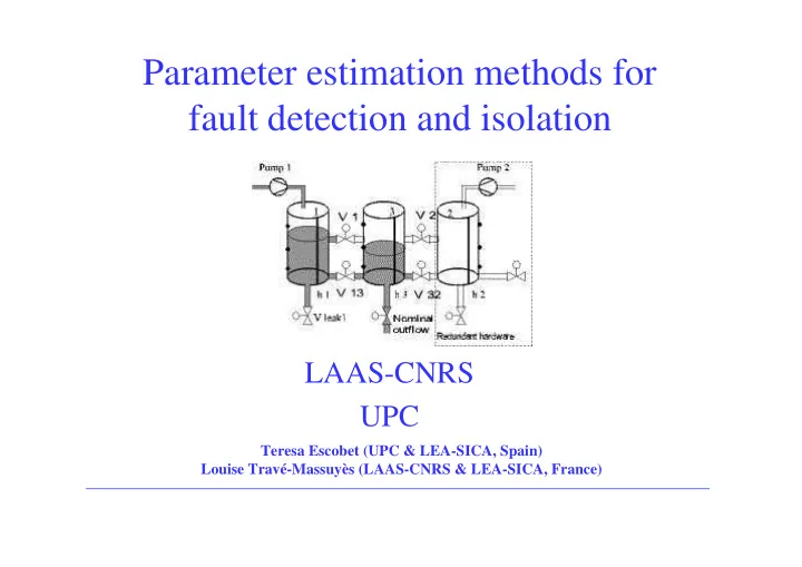
Parameter estimation methods for fault detection and isolation LAAS-CNRS UPC Teresa Escobet (UPC & LEA-SICA, Spain) Louise Travé-Massuyès (LAAS-CNRS & LEA-SICA, France)

Parameter estimation methods for fault detection and isolation Teresa Escobet Louise Travé-Massuyès (UPC & LEA-SICA, Spain) (LAAS-CNRS & LEA-SICA, France) March, 7-9 DX 2001 2 Via Lattea, Italian Alps

March, 7-9 DX 2001 3 Via Lattea, Italian Alps

e u θ y Parameter Estimation θ Calculation of Theoretical modeling p= f -1 ( θ ) process coefficients p Changes ∆ p, ∆θ ∆ p, ∆θ Fault decision March, 7-9 DX 2001 4 Via Lattea, Italian Alps

Parameter estimation for fault detection Recursive Least Squares algorithms = − + + − + − + + − − L L Input-output model: y ( t ) a y ( t 1 ) a y ( t n ) b u ( t n ) b u ( t n n ) 1 n a 1 k n b k a b Recursive Least Squares algorithm: − ϕ P ( t 1 ) ( t ) = k ( t ) + ϕ − ϕ T 1 ( t ) P ( t 1 ) ( t ) = − − ϕ − T P ( t ) P ( t 1 ) k ( t ) ( t ) P ( t 1 ) ) ε = − ϕ θ − T ( t ) y ( t ) ( t ) ( t 1 ) ) ) θ = θ − + ε ( t ) ( t 1 ) k ( t ) ( t ) [ ] ϕ = − − − − − − − where: T K K ( t ) y ( t 1 ) y ( t n ) u ( t nk ) u ( t n nk ) a b [ ] θ = T K K a a b b 1 n 1 n a b March, 7-9 DX 2001 5 Via Lattea, Italian Alps

Parameter estimation for fault detection Recursive Least Squares algorithms characteristics • The algorithm needs initial values: θ (0) and P (0) N � •The result minimises the expression: θ = ε 2 V ( ) ( t ) N = 1 t •LS estimate is consistent when: E { ϕ (t) ϕ T (t) } is non singular & E { ϕ (t) ε (t) } = 0 •The convergence speed is generally slow. •Approaches for modifying the RLS algorithm to make it suitable as a real-time fault detection method: Use of a forgetting factor Use of a virtual Kalman filter Use of sliding window data March, 7-9 DX 2001 6 Via Lattea, Italian Alps

Parameter estimation for fault detection Forgetting factor N � θ = λ − ε The loss function to be minimized: t s 2 V ( ) ( s ) N = s 1 − ϕ P ( t 1 ) ( t ) The RLS method with forgetting = k ( t ) λ + ϕ − ϕ T ( t ) P ( t 1 ) ( t ) factor is: ( ) 1 = − − ϕ − T P ( t ) P ( t 1 ) k ( t ) ( t ) P ( t 1 ) λ ) ε = − ϕ θ − T ( t ) y ( t ) ( t ) ( t 1 ) ) ) θ = θ − + ε ( ) ( 1 ) ( ) ( ) t t k t t Characteristics: •The parameter estimates converge to their true value quicker, thus decreasing the fault alarm delay time •But at the expense of increased sensitivity to noise. If λ is much less than 1 the estimates may even oscillates around their true value March, 7-9 DX 2001 7 Via Lattea, Italian Alps

Parameter estimation for fault detection Forgetting factor- Approaches • Time-varying forgetting factor [Fortescue et al. 1981] ) = ϕ − θ − T 1 . Prediction y ( t ) ( t 1 ) ( t 1 ) ˆ ε = − 2 . Error ( t ) y ( t ) y ( t ) ˆ − ϕ P ( t 1 ) ( t ) = 3 . Gain k ( t ) + ϕ − ϕ T 1 ( t ) P ( t 1 ) ( t ) ( ) λ = − − ϕ − ε σ T 2 4 . Forgetting ( t ) 1 1 ( t 1 ) k ( t ) ( t ) / 0 λ < λ = note : if them (t) ë (t) ë min min ( ) 1 = − − ϕ − T 5 . Covariance P ( t ) P ( t 1 ) k ( t ) ( t ) P ( t 1 ) λ ( ) t • The value of the constant σ 0 is the expected measurement noise variance which must be chosen based on the knowledge of the system. •The minimum value for λ (t) is also to be chosen by the user. March, 7-9 DX 2001 8 Via Lattea, Italian Alps

Parameter estimation for fault detection Forgetting factor- Approaches • Kalman filter { } + = + = δ T State equation: x ( t 1 ) x ( t ) v ( t ); E v ( t ) v ( s ) R 1 t , s − ϕ P ( t 1 ) ( t ) = Recursive k ( t ) + ϕ − ϕ T 1 ( t ) P ( t 1 ) ( t ) algorithm: ( ) = − − ϕ − + T P ( t ) P ( t 1 ) k ( t ) ( t ) P ( t 1 ) R 1 ) ε = − ϕ θ − T ( t ) y ( t ) ( t ) ( t 1 ) ) ) θ = θ − + ε ( t ) ( t 1 ) k ( t ) ( t ) • The covariance matrix R 1 has a similar role as the forgetting factor λ . • These design variable should be chosen by trade-off between fast detection (which requires λ “small” or R 1 “large”) and reliability (which requires λ close to 1 or R 1 “small”) March, 7-9 DX 2001 9 Via Lattea, Italian Alps

Benchmark process fault detection − − 1 1 b z b z ∆ = ∆ − ∆ 11 12 h ( z ) Q S The system can be modeled by: − − − − 1 n 1 1 1 a z 1 a z 1 1 − − 1 1 b z b z ∆ = ∆ − ∆ 21 22 h ( z ) h S − − − − 3 1 n 1 1 1 a z 1 a z 2 2 March, 7-9 DX 2001 10 Via Lattea, Italian Alps

Benchmark process fault detection Scenario I : a 2 a 1 valve V1 blocked closed from time 1000 b 11 b 21 b 12 b 22 March, 7-9 DX 2001 11 Via Lattea, Italian Alps

Benchmark process fault detection a 2 Scenario II : a 1 V1 blocked opened b 11 b 21 b 22 b 12 March, 7-9 DX 2001 12 Via Lattea, Italian Alps

Benchmark process fault detection Scenario III : a 1 a 2 leak in tank 1, the fault occurs at time 800 seconds b 11 b 21 b 12 b 22 March, 7-9 DX 2001 13 Via Lattea, Italian Alps

Conclusions • This benchmark is not ideal to test identification methods because two out of three of the proposed faults change the model structure • An advantage of these methods is to approach simultaneously the fault detection and fault isolation problems • A problem that must be reported about estimation methods is their high sensitivity to the parametrization, i.e. in our case, the values of λ and R1 • Our experiments show that the convergence rate of the algorithms is a critical issue March, 7-9 DX 2001 14 Via Lattea, Italian Alps