Overview Bayesian Methods for Parameter Estimation Introduction to - PowerPoint PPT Presentation

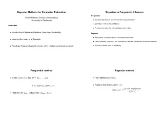
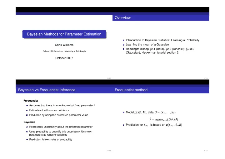
Overview Bayesian Methods for Parameter Estimation Introduction to Bayesian Statistics: Learning a Probability Learning the mean of a Gaussian Chris Williams Readings: Bishop §2.1 (Beta), §2.2 (Dirichlet), §2.3.6 School of Informatics, University of Edinburgh (Gaussian), Heckerman tutorial section 2 October 2007 1 / 18 2 / 18 Bayesian vs Frequentist Inference Frequentist method Frequentist Assumes that there is an unknown but fixed parameter θ Estimates θ with some confidence Model p ( x | θ, M ) , data D = { x 1 , . . . , x n } Prediction by using the estimated parameter value ˆ θ = argmax θ p ( D | θ, M ) Bayesian Prediction for x n + 1 is based on p ( x n + 1 | ˆ θ, M ) Represents uncertainty about the unknown parameter Uses probability to quantify this uncertainty. Unknown parameters as random variables Prediction follows rules of probability 3 / 18 4 / 18

Bayesian method Bayes, MAP and Maximum Likelihood Prior distribution p ( θ | M ) � Posterior distribution p ( θ | D , M ) p ( x n + 1 | D , M ) = p ( x n + 1 | θ, M ) p ( θ | D , M ) d θ p ( θ | D , M ) = p ( D | θ, M ) p ( θ | M ) p ( D | M ) Maximum a posteriori value of θ Making predictions θ MAP = argmax θ p ( θ | D , M ) � p ( x n + 1 | D , M ) = p ( x n + 1 , θ | D , M ) d θ Note: not invariant to reparameterization (cf ML estimator) � = p ( x n + 1 | θ, D , M ) p ( θ | D , M ) d θ If posterior is sharply peaked about the most probable value θ MAP then � p ( x n + 1 | D , M ) ≃ p ( x n + 1 | θ MAP , M ) = p ( x n + 1 | θ, M ) p ( θ | D , M ) d θ In the limit n → ∞ , θ MAP converges to ˆ θ (as long as p (ˆ θ ) � = 0) Interpretation: average of predictions p ( x n + 1 | θ, M ) Bayesian approach most effective when data is limited, n is small weighted by p ( θ | D , M ) Marginal likelihood (important for model comparison) 5 / 18 6 / 18 � Learning probabilities: thumbtack example Likelihood Frequentist Approach Likelihood for a sequence of heads and tails The probability of heads θ is unknown heads tails p ( hhth . . . tth | θ ) = θ n h ( 1 − θ ) n t Given iid data, estimate θ using an estimator MLE n h ˆ θ = with good properties n h + n t (e.g. ML estimator) 7 / 18 8 / 18

Learning probabilities: thumbtack example Examples of the Beta distribution 3.5 2 1.8 Bayesian Approach: (a) the prior 3 1.6 1.4 2.5 1.2 Prior density p ( θ ) , use beta distribution 2 1 0.8 1.5 0.6 0.4 1 p ( θ ) = Beta ( α h , α t ) ∝ θ α h − 1 ( 1 − θ ) α t − 1 0.2 0.5 0 0 0.1 0.2 0.3 0.4 0.5 0.6 0.7 0.8 0.9 1 0 0.1 0.2 0.3 0.4 0.5 0.6 0.7 0.8 0.9 1 Beta(0.5,0.5) Beta(1,1) for α h , α t > 0 1.8 4.5 Properties of the beta distribution 1.6 4 1.4 3.5 1.2 3 1 2.5 � α h 0.8 2 E [ θ ] = θ p ( θ ) = 0.6 1.5 α h + α t 0.4 1 0.2 0.5 0 0 0 0.1 0.2 0.3 0.4 0.5 0.6 0.7 0.8 0.9 1 0 0.1 0.2 0.3 0.4 0.5 0.6 0.7 0.8 0.9 1 Beta(3,2) Beta(15,10) 9 / 18 10 / 18 Bayesian Approach: (c) making predictions Bayesian Approach: (b) the posterior θ p ( θ | D ) ∝ p ( θ ) p ( D | θ ) ∝ θ α h − 1 ( 1 − θ ) α t − 1 θ n h ( 1 − θ ) n t ∝ θ α h + n h − 1 ( 1 − θ ) α t + n t − 1 x x x x n+1 1 2 n Posterior is also a Beta distribution ∼ Beta ( α h + n h , α t + n t ) The Beta prior is conjugate to the binomial likelihood (i.e. � p ( X n + 1 = heads | D , M ) = p ( X n + 1 = heads | θ ) p ( θ | D , M ) d θ they have the same parametric form) � α h and α t can be thought of as imaginary counts, with = θ Beta (( α h + n h , α t + n t ) d θ α = α h + α t as the equivalent sample size = α h + n h α + n 11 / 18 12 / 18

Beyond Conjugate Priors Generalization to multinomial variables Dirichlet prior r θ α i − 1 � p ( θ 1 , . . . , θ r ) = Dir ( α 1 , . . . , α r ) ∝ i i = 1 The thumbtack came from a magic shop → a mixture prior with � θ i = 1 , α i > 0 i p ( θ ) = 0 . 4 Beta ( 20 , 0 . 5 ) + 0 . 2 Beta ( 2 , 2 ) + 0 . 4 Beta ( 0 . 5 , 20 ) α i ’s are imaginary counts, α = � i α i is equivalent sample size Properties E ( θ i ) = α i α Dirichlet distribution is conjugate to the multinomial likelihood 13 / 18 14 / 18 Inferring the mean of a Gaussian Posterior distribution r � θ α i + n i − 1 p ( θ | n 1 , . . . , n r ) ∝ Likelihood i i = 1 p ( x | µ ) ∼ N ( µ, σ 2 ) Marginal likelihood Prior p ( µ ) ∼ N ( µ 0 , σ 2 0 ) r Γ( α ) Γ( α i + n i ) � p ( D | M ) = Given data D = { x 1 , . . . , x n } , what is p ( µ | D ) ? Γ( α + n ) Γ( α i ) i = 1 15 / 18 16 / 18

Comparing Bayesian and Frequentist approaches p ( µ | D ) ∼ N ( µ n , σ 2 n ) with n x = 1 � x i Frequentist : fix θ , consider all possible data sets n i = 1 generated with θ fixed n σ 2 σ 2 Bayesian : fix D , consider all possible values of θ 0 µ n = 0 + σ 2 x + 0 + σ 2 µ 0 n σ 2 n σ 2 One view is that Bayesian and Frequentist approaches have different definitions of what it means to be a good 1 = n σ 2 + 1 estimator σ 2 σ 2 n 0 See Bishop §2.3.6 for details 17 / 18 18 / 18