Week 3: Linear Regression Instructor: Sergey Levine 1 The - PDF document
Week 3: Linear Regression Instructor: Sergey Levine 1 The regression problem We saw how we can estimate the parameters of probability distributions over a random variable x . However, in a supervised learning setting, we might be interested in
Week 3: Linear Regression Instructor: Sergey Levine 1 The regression problem We saw how we can estimate the parameters of probability distributions over a random variable x . However, in a supervised learning setting, we might be interested in predicting the value of some output variable y . For example, we might like to predict the salaries that CSE 446 students will receive when they graduate. In order to make an accurate prediction, we need some information about the students: we need some set of features . For example, we could try to predict the salaries that students will receive based on the grades they got on each homework assignment. Perhaps some assignments are more important to complete than others, or more accurately reflect the kinds of skills that employ- ers look for. This kind of problem can be framed as regression . Question. What is the data? Answer. Like with decision trees, the data consists of tuples ( x i , y i ). Except now, y ∈ R is continuous, as are all of the attributes (features) in the vector x . The dataset is given by D = { ( x 1 , y 1 ) , . . . , ( x N , y N ) } . What is the hypothesis space? Question. This is a design choice. A simple and often very powerful hypothesis Answer. space consists of linear functions on the feature vector x i , given by f ( x i ) = � d j =1 w j x i,j = x i · w . The parameters of this hypothesis are the weights w ∈ R d . Question. What is the objective? This is also a design choice. Intuitively, we would like f ( x i ) to be Answer. “close” to y i , so we can write our objective as: N � w ← arg min ˆ D ( f ( x i ) , y i ) , w i =1 where D ( a, b ) is some measure of distance. Which distance measure to use? Well, a popular choice is to simply use the ℓ 2 norm (squared error), given by 1
D ( f ( x i ) , y i ) = ( f ( x i ) − y i ) 2 . This gives us the following objective: N � ( f ( x i ) − y i ) 2 , w ← arg min ˆ w i =1 Given our definition of f ( x i ), this is simply N � ( x i · w − y i ) 2 , w ← arg min ˆ w i =1 As we will see later in the lecture, this choice of distance function corresponds to a kind of probabilistic model, which turns regression into a MLE problem. Question. What is the algorithm? Answer. Just like in the MLE lectures, we can derive the optimal ˆ w by taking the derivative of the objective and setting it to zero. Note that we take the derivative with respect to a vector quantity w (this is also called the gradient): N N d ( x i · w − y i ) 2 = � � x i ( x i · w − y i ) = 0 . d w i =1 i =1 So the gradient consists of the sum over all datapoints of the (signed) error (also called the residual), times the feature vector of that datapoint x i . To make it convenient to derive the solution w , we can rearrange this in matrix notation, by defining x T y 1 1 x T y 2 2 X = Y = . . . . . . x T y N N Then we can see that the summation in the gradient equation above can be equivalently expressed as a matrix product: N w − y i ) = X T ( X ˆ w − Y ) = X T X ˆ w − X T Y = 0 � x i ( x i · ˆ i =1 Now we can rearrange terms and solve for w with a bit of linear algebra: X T X ˆ w = X T Y ⇒ ˆ w = ( X T X ) − 1 X T Y . This gives us the optimal estimate ˆ w that minimizes the sum of squared errors. 2
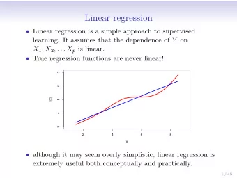
2 Features In machine learning, it is often useful for us to make a distinction between fea- tures and inputs. This is particularly true in the case of linear regression: since the function we are learning is linear, choosing the right features is important to get the necessary flexibility. For example, imagine that we want to predict salaries y for students in CSE 446. All we have is their grades on the home- works, arranged into a 4D vector x . If we learn a linear function of x , we will probably see that the higher the scores get, the higher the salaries. But what if in reality, there are diminishing returns: students who get bad scores get low salaries, but higher salaries don’t result in a proportional increase, since these scores are already “good enough” – the resulting function might look a little bit like a quadratic. So perhaps in this case, it would be really nice if we had some quadratic features. We can do this by defining a feature function h ( x i ). For example, if we want quadratic features, we might define: x i, 1 x 2 i, 1 x i, 2 x 2 i, 2 h ( x i ) = x i, 3 x 2 i, 3 x i, 4 x 2 i, 4 Let h i = f ( x i ), then we can write the linear regression problem in terms of the features h i as N � ( h i · w − y i ) 2 w ← arg min ˆ w i =1 We can then solve for the optimal ˆ w exactly the same way as before, only using H instead of X : w = ( H T H ) − 1 H T Y ˆ So we can see that in this way, we can use the same exact least squares objective and the same algorithm to fit a quadratic instead of a linear function. In general, we can fit any function that can be expressed as a linear combination of features. In the case of standard linear regression, expressed as f ( x i ) = Question. w · x i , what is the data, hypothesis space, objective, and algorithm? What is the data, hypothesis space, objective, and algorithm in the case where we have f ( x i ) = w · h ( x i ), where h ( . . . ) extracts linear and quadratic features? Answer. The data, objective, and algorithm are the same in both cases. The only thing that changes is the hypothesis space: in the former case, we have the class of all lines, and in the latter case, we have the class of all (diagonal) quadratic functions. 3
In fact, we can choose any class of features h ( x i ) we want to learn complex functions of the input. A few choices are very standard for linear regression and are used almost always. For example, we often want to include a constant feature, e.g. x i, 1 . . . h ( x i ) = x i,d 1 so that the linear regression weights w include a constant bias (which is simply the coefficient on the last, constant feature). 3 Linear regression as MLE At this point, we might wonder why we actually use the sum of squared errors as our objective. The choice seems reasonable, but a bit arbitrary. In fact, linear regression can be viewed as (conditional) maximum likelihood estimation under a particular simple probabilistic model. Unlike in the MLE examples covered last week, now our dataset D includes both inputs and outputs, since D = { ( x 1 , y 1 ) , ( x 2 , y 2 ) , . . . , ( x N , y N ) } . So we will aim to construct a conditional likelihood of the form p ( y | x , θ ). What kind of likelihood can we construct such that log p ( y | x , θ ) Question. corresponds to squared error? We saw last week that for continuous variables (such as y ), a good Answer. choice of distribution is the Gaussian distribution. Note that the logarithm of a Gaussian distribution is quadratic in the variable y : 1 2 σ 2 ( µ − y ) 2 + const . log p ( y | µ, σ ) = − log σ − That looks a lot like the squared error objective in linear regression – we just need to figure out how to design σ and µ . If we simply set µ = f ( x ), we get: 1 2 σ 2 ( x · w − y ) 2 + const . log p ( y | x , w , σ ) = − log σ − So the (conditional) log-likelihood of our entire dataset is given by N 1 ( x i · w − y i ) 2 + const . � L ( w , σ ) = − N log σ − 2 σ 2 i =1 If we set the derivative with respect to w to zero, we get N N − 1 � � x i ( x i · w − y i ) = 0 ⇒ x i ( x i · w − y i ) = 0 , 2 σ 2 i =1 i =1 4
which is exactly the same equation as what we saw for the sum of squared errors objective. Therefore, the solution under this model is given, as before, by w = ( X T X ) − 1 X T Y , ˆ and we can estimate the variance σ 2 by plugging in the optimal mean: N σ 2 = 1 � w − y ) 2 . ( x i · ˆ N i =1 However, σ 2 won’t affect the maximum likelihood prediction of y , which will always be x i · ˆ w , the most probable value according to the Gaussian model, so we often disregard σ 2 when performing linear regression. What is the practical, intuitive interpretation of this probabilistic model? This model states that the data comes from some underlying Gaussian distri- bution y ∼ N ( x · w , σ 2 ), so the samples we observe are noisy realizations of the underlying function x · w . Therefore, any deviation from this function is modeled as symmetric Gaussian noise. 5
Recommend
More recommend
Explore More Topics
Stay informed with curated content and fresh updates.
