Advanced Mathematical Methods Part II Statistics Generalised - PowerPoint PPT Presentation
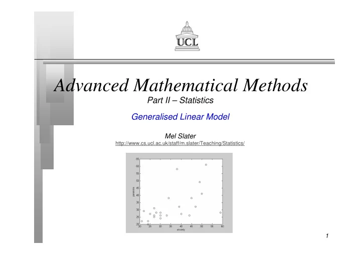
Advanced Mathematical Methods Part II Statistics Generalised Linear Model Mel Slater http://www.cs.ucl.ac.uk/staff/m.slater/Teaching/Statistics/ 1 Outline Introduction The General Linear Model Least Squares Estimation
Advanced Mathematical Methods Part II – Statistics Generalised Linear Model Mel Slater http://www.cs.ucl.ac.uk/staff/m.slater/Teaching/Statistics/ 1
Outline � Introduction � The General Linear Model � Least Squares Estimation � Hypothesis Testing � Analysis of Variance � Multiple Correlation 2
Statistical Relationship � Experiments are usually conducted to understand the relationship between a response variable y and a set of independent variables x 1 ,x 2 ,…,x k . � y is a random variable and the x’s are thought of as constants. � E(y) = f(x 1 ,x 2 ,…,x k ) 3
Linear Model � In practice the model is ‘linear’ • The linearity refers to linearity in the parameters (not in the x’s) � We have observations on n individuals, and, another way to write this is: 4
Matrix Representation � y = X β + ε • A more succinct form • y is an n*1 vector • X is a n*p matrix (of constants) • β is a p*1 vector • ε is an n*1 vector of random variables � Note that p=k+1 if a constant term β 0 is included and the first column of X consists of 1s. � Normally there should be a constant term. 5
Problems � To estimate the unknown parameters β � To make inferences about β � In particular we can find confidence intervals for β � We can test hypotheses, in particular the hypotheses • H 0 : β 1 = β 2 = …= β k = 0 (null hypothesis) • H 1 : at least one β j ≠ 0 – Tests for relationship between y and X. 6
Least Squares Solution � β * = (X T X) -1 X T y • This is the L.S. solution • Minimises the sum of squares of errors between the fitted values and the true values of y. � E( β *) = β � Var( β *) = σ 2 (X T X) -1 • Where Var( ε ) = σ 2 I 7
Analysis of Variance = ∑ � The total variation in the n i − 2 TSS y y ( ) response variable is = i 1 • It is the sample variance without dividing by n-1 � Let y* = X β * • This is the fitted or predicted response = ∑ n � Then the total variation in i − 2 FSS ( y * y ) the fitted variable is = i 1 8
Analysis of Variance � The residual SS is defined as: • RSS = TSS - FSS • It is what is ‘unexplained’ by the model � If the model fitted the data then • FSS = TSS and RSS = 0 9
Analysis of Variance � Now we make the further assumption that ε ~ N(0, σ 2 I) � Then under this assumption and the null hypothesis: • FSS / σ 2 ~ Chi-squared (k) • RSS / σ 2 ~ Chi-squared (n-k) • And MFSS and MRSS are independent � F = FSS/RSS ~ F(k,n-k) • Large F should reject the null hypothesis 10
Analysis of Variance Table Source df SS MSS F- Ratio X vars k Fitted Fitted/k MFSS / MRSS Residual n-k Residual= Res/(n-k) deviance Total n-1 Total 11
Multiple Correlation � R 2 = Fitted SS/ Total SS � This is the multiple correlation coefficient � It is the proportion of the variation in the response variable that is explained by the model. � R 2 is between 0 and 1 � It should be used together with the F- Ratio to determine significance of the model 12
Testing individual β � Each β * ~ t-distribution on n-k degrees of freedom, on the null hypothesis that β =0 � This can be used to construct confidence intervals or tests of significance � An approx rule is if β * / SE( β *) >2 reject null hypothesis • � The ‘standard deviation’ for an estimate is often called the ‘standard error’ (SE). 13
Estimating σ 2 � An unbiased estimator for σ 2 is s 2 • s 2 = MRSS (mean residual SS) � Therefore • SE-squared( β *) = s 2 (X T X) -1 14
Using GLIM � $units 24 !the number of obs � $data x1 x2 x3 y !variables � $read � !data follows this in logical row order � !data goes here � $finish !marks the end of the file � Suppose the file name is file.txt 15
Using GLIM � $input 10 132 !reads in the file with maximum field width of 132 chars • Yes this is a very old system!!!! � $yvar y !declare which variable is the response � $fit x1+x2+x3 !will fit the regression model 16
Using GLIM � GLIM will print out the deviance and degrees of freedom • Deviance = residual sum of squares of the model • D.f. = degrees of freedom of the residual � Note if you fit the empty model, it will just fit a constant term: • $fit $ !fits the model y = beta0 � The deviance for this is the Total SS 17
Using GLIM � $display e !will print out the estimates of beta and their standard errors � This can be used to look at each beta individually and assess its utility � The higher the ratio • estimate/SE � the better that parameter and the more that the corresponding x contributes to y. 18
Using GLIM � You can incrementally fit variables • $fit +x4 $!adds x4 to the model � $fit . $ !refits the current model � $display m $!displays the current model � The advantage of GLIM compared to MATLAB is that you don’t need to specify explicitly the X matrix � The ‘user interface’ is the disadvantage 19
Comparing Two Models � Suppose you have fitted a model • $fit x1+x2+x3 !model S1 � You want to see if adding more terms makes a significant difference eg • $fit +x4+x5 !model S2 � Is S2 better than S1? 20
Comparing Two Models � Take the F-Ratio ∆ ∆ deviance / df = ∆ F ~ F ( df , df ( S 2 )) MRSS ( S 2 ) � If this is large then reject the null hypothesis that the additional variables make no difference. 21
Recommend
More recommend
Explore More Topics
Stay informed with curated content and fresh updates.
