Week 1: Introduction, Simple Linear Regression Data visualization, - PowerPoint PPT Presentation
BUS 41100 Applied Regression Analysis Week 1: Introduction, Simple Linear Regression Data visualization, conditional distributions, correlation, and least squares regression Max H. Farrell The University of Chicago Booth School of Business
BUS 41100 Applied Regression Analysis Week 1: Introduction, Simple Linear Regression Data visualization, conditional distributions, correlation, and least squares regression Max H. Farrell The University of Chicago Booth School of Business
The basic problem Formulate a model to Available Use estimate data on predict or to make a two or more estimate a (business) variables value of decision interest 1
Regression: What is it? ◮ Simply: The most widely used statistical tool for understanding relationships among variables ◮ A conceptually simple method for investigating relationships between one or more factors and an outcome of interest ◮ The relationship is expressed in the form of an equation or a model connecting the outcome to the factors 2
Regression in business ◮ Optimal portfolio choice: - Predict the future joint distribution of asset returns - Construct an optimal portfolio (choose weights) ◮ Determining price and marketing strategy: - Estimate the effect of price and advertisement on sales - Decide what is optimal price and ad campaign ◮ Credit scoring model: - Predict the future probability of default using known characteristics of borrower - Decide whether or not to lend (and if so, how much) 3
Regression in everything Straight prediction questions: ◮ What price should I charge for my car? ◮ What will the interest rates be next month? ◮ Will this person like that movie? Explanation and understanding: ◮ Does your income increase if you get an MBA? ◮ Will tax incentives change purchasing behavior? ◮ Is my advertising campaign working? 4
Data Visualization Example: pickup truck prices on Craigslist We have 4 dimensions to consider. > data <- read.csv("pickup.csv") > names(data) [1] "year" "miles" "price" "make" A simple summary is > summary(data) year miles price make Min. :1978 Min. : 1500 Min. : 1200 Dodge:10 1st Qu.:1996 1st Qu.: 70958 1st Qu.: 4099 Ford :12 Median :2000 Median : 96800 Median : 5625 GMC :24 Mean :1999 Mean :101233 Mean : 7910 3rd Qu.:2003 3rd Qu.:130375 3rd Qu.: 9725 Max. :2008 Max. :215000 Max. :23950 5
First, the simple histogram (for each continuous variable). > par(mfrow=c(1,3)) > hist(data$year) > hist(data$miles) > hist(data$price) Histogram of data$year Histogram of data$miles Histogram of data$price 15 15 20 15 10 10 Frequency Frequency Frequency 10 5 5 5 0 0 0 1975 1980 1985 1990 1995 2000 2005 2010 0 50000 100000 150000 200000 250000 0 5000 10000 15000 20000 25000 data$year data$miles data$price Data is “binned” and plotted bar height is the count in each bin. 6
We can use scatterplots to compare two dimensions. > par(mfrow=c(1,2)) > plot(data$year, data$price, pch=20) > plot(data$miles, data$price, pch=20) ● ● ● ● ● ● ● ● 15000 15000 ● ● data$price data$price ● ● ● ● ● ● ● ● ● ● ● ● ● ● ● ● ● ● ● ● ● ● ● ● ● ● ● ● ● ● 5000 ● 5000 ● ● ● ● ● ● ● ● ● ● ● ● ● ● ● ● ● ● ●● ● ● ● ● ● ● ● ● ● ● ● ● ● ● ● ● ● ● ● ● ● ● ● ● ● ● ● ● ● ● ● 1980 1990 2000 0 50000 150000 data$year data$miles 7
Add color to see another dimension. > par(mfrow=c(1,2)) > plot(data$year, data$price, pch=20, col=data$make) > legend("topleft", levels(data$make), fill=1:3) > plot(data$miles, data$price, pch=20, col=data$make) ● ● Dodge Ford ● ● ● ● GMC ● ● 15000 15000 ● ● data$price data$price ● ● ● ● ● ● ● ● ● ● ● ● ● ● ● ● ● ● ● ● ● ● ● ● ● ● ● ● ● ● 5000 ● 5000 ● ● ● ● ● ● ● ● ● ● ● ● ● ● ● ● ● ● ●● ● ● ● ● ● ● ● ● ● ● ● ● ● ● ● ● ● ● ● ● ● ● ● ● ● ● ● ● ● ● ● 1980 1990 2000 0 50000 150000 data$year data$miles 8
Boxplots are also super useful. > year_boxplot <- factor(1*(year<1995) + 2*(1995<=year & year<2000) + 3*(2000<=year & year<2005) + 4*(2005<=year & year<2009), labels=c("<1995", "’95-’99", "2000-’04", "’05-’09")) > boxplot(price ~ make, ylab="Price ($)", main="Make") > boxplot(price ~ year_boxplot, ylab="Price ($)", main="Year") Make Year ● 15000 15000 Price ($) Price ($) ● ● 5000 5000 ● Dodge Ford GMC <1995 '95−'99 2000−'04 '05−'09 The box is the Interquartile Range (IQR; i.e., 25 th to 75 th %), with the median in bold. The whiskers extend to the most extreme point which is 9 no more than 1.5 times the IQR width from the box.
Regression is what we’re really here for. > plot(data$year, data$price, pch=20, col=data$make) > abline(lm(price ~ year),lwd=1.5) ● ● Dodge Ford ● ● ● ● GMC ● ● 15000 15000 ● ● data$price data$price ● ● ● ● ● ● ● ● ● ● ● ● ● ● ● ● ● ● ● ● ● ● ● ● ● ● ● ● ● ● 5000 ● 5000 ● ● ● ● ● ● ● ● ● ● ● ● ● ● ● ● ● ● ●● ● ● ● ● ● ● ● ● ● ● ● ● ● ● ● ● ● ● ● ● ● ● ● ● ● ● ● ● ● ● ● 1980 1990 2000 0 50000 150000 data$year data$miles ◮ Fit a line through the points, but how? ◮ lm stands for l inear m odel ◮ Rest of the course: formalize and explore this idea 10
Conditional distributions Regression models are really all about modeling the conditional distribution of Y given X . Why are conditional distributions important? We want to develop models for forecasting. What we are doing is exploiting the information in the conditional distribution of Y given X . The conditional distribution is obtained by “slicing” the point cloud in the scatterplot to obtain the distribution of Y conditional on various ranges of X values. 11
Conditional v. marginal distribution Consider a regression of house price on size: “slice” of data { ● ● ● ● 400 ● ● ● ● ● ● ● ● ● ● ● ● ● ● ● ● ● ● ● ● ● ● ● ● ● ● ● ● ● ● ● ● ● ● ● ● ● ● ● ● ● ● ● ● ● ● ● ● ● ● ● ● ● ● 300 ● ● ● ● ● ● ● ● ● ● ● ● ● ● ● ● ● ● ● ● ● ● ● ● ● ● ● ● ● ● ● ● ● ● ● ● ● ● price ● ● ● ● ● ● ● ● ● ● ● ● ● ● ● ● ● ● ● ● ● ● ● ● ● ● ● ● ● ● ● ● ● ● ● ● ● ● ● ● ● ● ● ● ● ● ● 200 ● ● ● ● ● ● ● ● ● ● ● ● ● ● ● ● ● ● ● ● ● ● ● ● ● ● ● ● ● ● ● ● ● ● ● ● ● ● ● ● ● ● ● ● ● ● ● ● ● ● conditional 100 ● marginal ● ● ● ● ● distribution ● distribution of price given 0.5 1.0 1.5 2.0 2.5 3.0 3.5 of price 3 < size < 3.5 size 400 ● 300 ● price ● 200 ● 100 regression line marg 1 − 1.5 1.5 − 2 2 − 2.5 2.5 − 3 3 − 3.5 12
Key observations from these plots: ◮ Conditional distributions answer the forecasting problem: if I know that a house is between 1 and 1.5 1000 sq.ft., then the conditional distribution (second boxplot) gives me a point forecast (the mean) and prediction interval. ◮ The conditional means (medians) seem to line up along the regression line. ◮ The conditional distributions have much smaller dispersion than the marginal distribution. 13
This suggests two general points: ◮ If X has no forecasting power, then the marginal and conditionals will be the same. ◮ If X has some forecasting information, then conditional means will be different than the marginal or overall mean and the conditional standard deviation of Y given X will be less than the marginal standard deviation of Y . 14
Recommend
More recommend
Explore More Topics
Stay informed with curated content and fresh updates.
