Unit 6: Introduction to linear regression 2. Outliers and inference - PowerPoint PPT Presentation

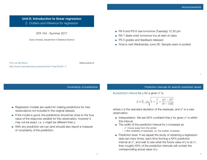
Announcements Unit 6: Introduction to linear regression 2. Outliers and inference for regression ▶ PA 6 and PS 6 due tomorrow (Tuesday) 12.30 pm STA 104 - Summer 2017 ▶ RA 7 (laste one!) tomorrow too at start of class Duke University, Department of Statistical Science ▶ PS 5 grades and feedback released ▶ Final is next Wednesday June 28: Sample exam is posted Prof. van den Boom Slides posted at http://www2.stat.duke.edu/courses/Summer17/sta104.001-1/ 1 Uncertainty of predictions Prediction intervals for specific predicted values A prediction interval for y for a given x ⋆ is √ n + ( x ⋆ − ¯ x ) 2 1 + 1 y ± t ⋆ n − 2 s ˆ ( n − 1) s 2 x ▶ Regression models are useful for making predictions for new where s is the standard deviation of the residuals, and x ⋆ is a new observations not included in the original dataset. observation. ▶ If the model is good, the predictions should be close to the true y for given x ⋆ is within ▶ Interpretation: We are XX% confident that ˆ value of the response variable for this observation, however it this interval. may not be exact, i.e. ˆ y might be different than y . ▶ The width of the prediction interval for ˆ y increases as ▶ With any prediction we can (and should) also report a measure – x ⋆ moves away from the center of uncertainty of the prediction. – s (the variability of residuals), i.e. the scatter, increases ▶ Prediction level: If we repeat the study of obtaining a regression data set many times, each time forming a XX% prediction interval at x ⋆ , and wait to see what the future value of y is at x ⋆ , then roughly XX% of the prediction intervals will contain the corresponding actual value of y . 2 3

3.378776 43.064 3.638e-06 *** Analysis of Variance Table 1.740003 Df Sum Sq Mean Sq F value Pr(>F) perc_pov 1 1308.34 1308.34 Residuals 18 1 0.7052275 546.86 30.38 confint(m_mur_pov, level = 0.95) 2.5 % 97.5 % (Intercept) -46.265631 -13.536694 perc_pov anova(m_mur_pov) Response: annual_murders_per_mil r_sq 1 21.28663 9.418327 33.15493 # predict summarise(r_sq = cor(annual_murders_per_mil, perc_pov)^2) murder %>% predict(m_mur_pov, newdata, interval = "prediction", level = 0.95) fit lwr upr (1) R 2 assesses model fit -- higher the better Calculating the prediction interval ▶ R 2 : percentage of variability in y explained by the model. ▶ For single predictor regression: R 2 is the square of the correlation coefficient, R . By hand: Don’t worry about it... In R: ▶ For all regression: R 2 = SS reg SS tot We are 95% confident that the annual murders per million for a county with 20% poverty rate is between 9.52 and 33.15. R 2 = explained variabilty = SS reg 1308 . 34 + 546 . 86 = 1308 . 34 1308 . 34 = 1855 . 2 ≈ 0 . 71 total variability SS tot 4 5 Inference for regression uses the t -distribution Clicker question 40 ● ▶ Use a T distribution for inference on the slope, with degrees of R 2 for the regression model for predicting ● 35 ● annual murders per million freedom n − 2 30 ● annual murders per million based on ● ● ● 25 ● – Degrees of freedom for the slope(s) in regression is df = n − k − 1 ● 20 ● percentage living in poverty is roughly 71%. ● where k is the number of slopes being estimated in the model. 15 ● ● ● ● ● Which of the following is the correct ● 10 ● ● ▶ Hypothesis testing for a slope: H 0 : β 1 = 0 ; H A : β 1 ̸ = 0 5 ● interpretation of this value? 14 16 18 20 22 24 26 – T n − 2 = b 1 − 0 % in poverty SE b 1 – p-value = P(observing a slope at least as different from 0 as the one (a) 71% of the variability in percentage living in poverty is explained observed if in fact there is no relationship between x and y by the model. ▶ Confidence intervals for a slope: (b) 84% of the variability in the murder rates is explained by the – b 1 ± T ⋆ n − 2 SE b 1 model, i.e. percentage living in poverty. – In R: (c) 71% of the variability in the murder rates is explained by the model, i.e. percentage living in poverty. (d) 71% of the time percentage living in poverty predicts murder rates accurately. 6 7

Conditions for regression Checking conditions Important regardless of doing inference 2000 ▶ Linearity → randomly scattered residuals around 0 in the 1000 residual plot – important regardless of doing inference Clicker question What condition is this linear model 0 obviously and definitely violating? Important for inference −1000 ▶ Nearly normally distributed residuals → histogram or normal (a) Linear relationship probability plot of residuals −2000 (b) Non-normal residuals ▶ Constant variability of residuals ( homoscedasticity ) → no fan (c) Constant variability shape in the residual plot 2000 (d) Independence of observations ▶ Independence of residuals (and hence observations) → depends on data collection method, often violated for 0 time-series data −2000 8 9 Checking conditions Type of outlier determines how it should be handled 2000 ▶ Leverage point is away from the cloud of points horizontally, does 1500 Clicker question not necessarily change the slope What condition is this linear model ▶ Influential point changes the 1000 obviously and definitely violating? slope (most likely also has high 500 leverage) – run the regression (a) Linear relationship with and without that point to 0 (b) Non-normal residuals determine (c) Constant variability −500 ▶ Outlier is an unusual point without these special characteristics 1000 (d) Independence of observations (this one likely affects the intercept only) ▶ If clusters (groups of points) are apparent in the data, it might be 0 worthwhile to model the groups separately. −1000 10 11

Summary of main ideas 1. Predicted values also have uncertainty around them Application exercise: 6.2 Linear regression 2. R 2 assesses model fit – higher the better See course website for details 3. Inference for regression uses the t -distribution 4. Conditions for regression 5. Type of outlier determines how it should be handled 12 13