Statistical Inference Fall 2018 Tyson S. Barrett, PhD The Whole - PowerPoint PPT Presentation
EDUC 7610 Chapter 4 Statistical Inference Fall 2018 Tyson S. Barrett, PhD The Whole Idea All can be done in R Why Statistical Inference? So far, weve used regression just to describe our sample But our goal is to understand the
EDUC 7610 Chapter 4 Statistical Inference Fall 2018 Tyson S. Barrett, PhD
The Whole Idea All can be done in R
Why Statistical Inference? So far, we’ve used regression just to describe our sample But our goal is to understand the population, not just our sample There is a “true” value out there in the population But we don’t have access to it (unless we use a census) • So we estimate it using our sample
Why Statistical Inference? Is our sample going to be exactly identical to the population we pulled it from?
Why Statistical Inference? Is our sample going to be exactly identical to the population we pulled it from? Sampling Variance (Error) Causes uncertainty in our estimates
To infer about the population, we need to make some assumptions 1 2 Homoscedasticity – the Linearity – the relationship conditional distributions of Y between outcome and have equal variances predictors is approx. linear 3 4 Independent Sampling – each Conditional Distribution of Y – member of our sample is is normally distributed independent of the other members
Linearity Linear Non − Linear (Square Root) Non − Linear (Squared) 20 200 8 15 150 value 100 6 10 50 5 4 0 2.5 5.0 7.5 10.0 2.5 5.0 7.5 10.0 2.5 5.0 7.5 10.0 x
Homoscedasticity Heteroscedastic Homoscedastic 50 60 40 30 40 value 20 20 10 0 0 5 10 15 20 5 10 15 20 x
Conditional Distribution of Y At each point of x, there is an assumed normal distribution around the line Central Limit Theorem helps us here (samples above 30 don’t rely on this assumption as much)
Independent Sampling Each member of our sample (e.g., person, class, animal) must be independent of the others No influence from one member to another • Name some situations where this would be violated When this is violated, we can use multilevel modeling techniques
What about violations of these assumptions? 1 2 Linearity – if this is violated we Homoscedasticity – can mess can try different specifications with your standard errors; can (e.g., square or square root of a use special estimators (sandwich predictor); otherwise, violating estimator, robust SEs) this is disastrous 3 4 Independent Sampling – can Conditional Distribution of Y – sometimes really mess up your often not too bad in larger results (simpson’s paradox); use samples multilevel modeling to fix
Assumptions Residuals vs Fitted Normal Q − Q and Residuals 11 11 62 62 2 2 Standardized residuals 1 1 Residuals 0 0 All of the assumptions can − 1 − 1 − 2 be framed in terms of the − 2 39 39 5 10 15 20 − 2 − 1 0 1 2 residuals Fitted values Theoretical Quantiles Residuals are normal, Scale − Location Residuals vs Leverage 1.5 11 homoscedastic, have a mean 39 62 2 87 Standardized residuals Standardized residuals of zero at all points of x, and 1.0 1 0 are uncorrelated 0.5 − 1 Cook's distance = i.i.d. (independently and identically − 2 68 6 0.0 distributed) 5 10 15 20 0.00 0.02 0.04 0.06 Fitted values Leverage
Quick Aside about Vocab and Notation If we did something a thousand times, what value do we expect? Expected Value !($ % ) !(") ! " An estimate that arrives at the Unbiased Estimation expected value ' = 1 ! " * +" '
Quick Aside about Vocab and Notation Is the following unbiased? Regression is an UNBIASED estimator of the population # = 1 ! " & '" # + 1 value We could show this mathematically No. If we did this many, many times, on average we’d be off by 1
Ordinary Least Squares Regression is B.L.U.E. It is the most precise (the smallest accurate standard errors) B est It is unbiased (it estimates the It is a linear model L inear population value) U nbiased Everything we are E stimator doing with regression is an estimate Note: Maximum likelihood regression is very similar
So what does all this mean? Regression provides us with the “best” linear, accurate way to understand a population using a sample
Regression Results in ANOVA form Regression results often are lead by an ANOVA table or information from an ANOVA table Remember that ANOVA is just a special case of regression?
What do we want to be able to infer? 1 Multiple R (or R 2 ) 2 Regression Coefficients 3 (Partial) Correlation
Inference: Multiple R This tests the entire model Do the predictor(s) together have a relationship with the outcome? • Common to discuss the model as a whole before discussing the individual • predictors Statistic of Interest Test Statistic Significance Example P < .05 suggests The model that included there is a SES explained 30% more of F-statistic relationship the variance in the R 2 (or adjusted R 2 ) among the outcome and was #$ %&' ! = predictor(s) significantly better (p < #$ %&( and outcome .001)
Inference: Multiple R The Null Hypothesis: Model is no better than comparison model (either a null model or another ”nested” model) The Alternative: Model is better than comparison Statistic of Interest Test Statistic Significance Another Example P < .05 suggests The model explained 45% there is a F-statistic of the variation in the relationship R 2 (or adjusted R 2 ) outcome and is significantly among the #$ %&' better than the null model ! = predictor(s) #$ %&( (p = .002). and outcome
Inference: Regression Coefficients This testing each individual predictor Do each predictor have a relationship with the outcome? • Most common way of interpreting regression • Statistic of Interest Test Statistic Significance Example P < .05 suggests Controlling for the there is a covariates, for a one unit relationship b j or ! T-statistic increase in SES, there is an " among this associated decrease of b 1 in predictor and the outcome (p = .03). the outcome
Inference: Regression Coefficients This testing each individual predictor Do each predictor have a relationship with the outcome? • Most common way of interpreting regression • We do the same tests for the standardized coefficients as well (just with standardized variables instead of the raw ones)
Inference: Regression Coefficients This testing each individual predictor Do each predictor have a relationship with the outcome? • Most common way of interpreting regression • Statistic of Interest Test Statistic Significance Example P < .05 suggests Controlling for the We do the same tests for the standardized there is a covariates, for a one SD coefficients as well (just with standardized relationship increase in SES, there is an b j or ! T-statistic " among this associated decrease of b 1 variables) predictor and SDs in the outcome (p = the outcome .03).
Inference: Regression Coefficients Important Pieces of the Coefficients • The Estimate • The Standard Error of the Estimate • Testing the null hypothesis • Confidence Intervals
Inference: Regression Coefficients The Estimate Simple $ = ,-.(', +) # 234(') Multiple $ % = ' ( ' )* ' ( + all #
Inference: Regression Coefficients estimate of variance of The Standard Error the residuals (! )*+,-./0 !"($ % ) = 9 ) (1) 234 5 % (1 − 8 9 here is the % 8 % R 2 from the model with all Sample size variables but j used in analysis this is called the Variance of that predictor tolerance
Inference: Regression Coefficients The Standard Error (! )*+,-./0 !"($ % ) = 9 ) (1) 234 5 % (1 − 8 % 234 5 (! )*+,-./0 % What increases the SE? 9 ) (1 − 8 1 %
Inference: Regression Coefficients The Standard Error 9 ) = The Tolerance of X j (1 − 8 % (! )*+,-./0 !"($ % ) = A measure of the independence of X j from the 9 ) (1) 234 5 % (1 − 8 % other predictors (i.e., measures the collinearity ) When Tol = 0, there is perfect collinearity • When 1 > Tol > 0, there is some correlation between • predictors When Tol = 1, there is no correlation at all between • predictors
Inference: Regression Coefficients The Standard Error 9 ) = The Tolerance of X j (1 − 8 % (! )*+,-./0 !"($ % ) = A measure of the independence of X j from the 9 ) (1) 234 5 % (1 − 8 % other predictors (i.e., measures the collinearity ) 1 Variance InBlation Factor % = 9 1 − 8 %
Inference: Regression Coefficients The Standard Error (! )*+,-./0 !"($ % ) = 9 ) (1) 234 5 % (1 − 8 % (! )*+,-./0 !"($ % ) = 2:; % ∗ (1) 234 5 %
The Standard Error when VIF 0.3 (or R j2 ) is increased 0.2 SE ( b j ) 0.1 VIF = 10 VIF = 5 VIF = 1.1 VIF = 1.4 VIF = 1.7 VIF = 2 VIF = 2.5 VIF = 3.3 VIF = 1 VIF = 1.2 0.0 0.00 0.25 0.50 0.75 1.00 2 R j
Inference: Regression Coefficients Using the Standard Error we can now do two important things Null Hypothesis Test Confidence Interval ! = # $ − null value of # 23 = # $ ± ! 5/7 ∗ ./(# $ ) $ ./(# $ ) Using either we can test the null hypothesis and make inferences about the population
Recommend
More recommend
Explore More Topics
Stay informed with curated content and fresh updates.
