Modes of Statistical Inference for Causal Efgects Plus an overview - PowerPoint PPT Presentation

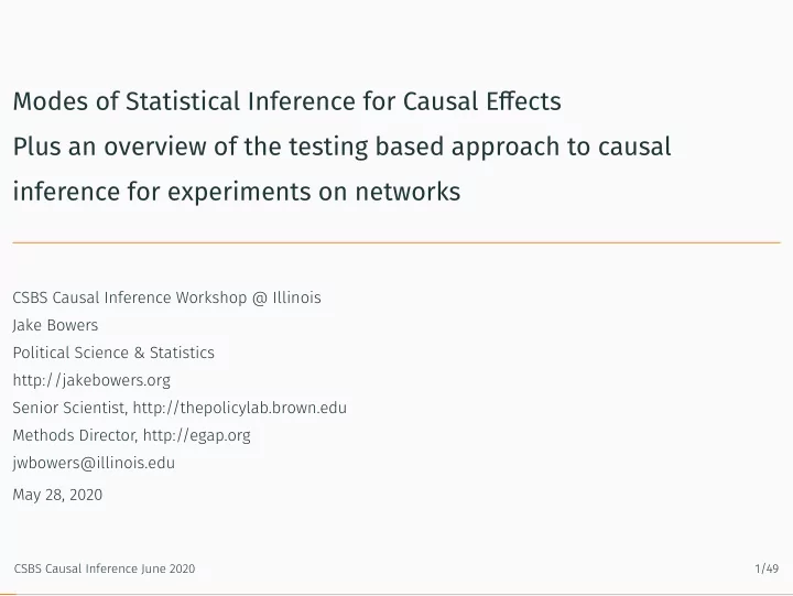
Modes of Statistical Inference for Causal Efgects Plus an overview of the testing based approach to causal inference for experiments on networks CSBS Causal Inference Workshop @ Illinois Jake Bowers Political Science & Statistics http://jakebowers.org Senior Scientist, http://thepolicylab.brown.edu Methods Director, http://egap.org jwbowers@illinois.edu May 28, 2020 CSBS Causal Inference June 2020 1/49

CSBS Causal Inference June 2020 2/49

An overview of approaches to statistical inference for causal quantities

Three General Approaches To Learning About The Unobserved Using Data CSBS Causal Inference June 2020 3/49

Three Approaches To Causal Inference: Potential Outcomes Imagine we would observe so many bushels of corn, 𝑧 , if plot 𝑗 were randomly assigned to new fertilizer, 𝑧 𝑗,𝑎 𝑗 =1 (where 𝑎 𝑗 = 1 means “assigned to new fertilizer” and 𝑎 𝑗 = 0 means “assigned status quo fertilizer”) and another amount of corn, 𝑧 𝑗,𝑎 𝑗 =0 , if the same plot were assigned the status quo fertilizer condition. These 𝑧 are are potential or partially observed outcomes. CSBS Causal Inference June 2020 4/49

• In a two arm experiment each unit has at least a pair of potential outcomes (𝑧 𝑗,𝑎 𝑗 =1 , 𝑧 𝑗,𝑎 𝑗 =0 ) (also written (𝑧 𝑗,1 , 𝑧 𝑗,0 ) to indicate that 𝑧 1,𝑎 1 =1,𝑎 2 =1 = 𝑧 1,𝑎 1 =1,𝑎 2 =0 ) • Causal Efgect for unit 𝑗 is 𝜐 𝑗 , 𝜐 𝑗 = 𝑔(𝑧 𝑗,1 , 𝑧 𝑗,0 ) . For example, 𝜐 𝑗 = 𝑧 𝑗,1 − 𝑧 𝑗,0 . • Fundamental Problem of (Counterfactual) Causality We only see one potential outcome 𝑍 𝑗 = 𝑎 𝑗 ∗ 𝑧 𝑗,1 + (1 − 𝑎 𝑗 )𝑧 𝑗,0 manifest in our observed outcome, 𝑍 𝑗 . Treatment reveals one potential outcome to us in a simple randomized experiment. Three Approaches To To Causal Inference: Notation • Treatment 𝑎 𝑗 = 1 for treatment and 𝑎 𝑗 = 0 for control for units 𝑗 CSBS Causal Inference June 2020 5/49

• Causal Efgect for unit 𝑗 is 𝜐 𝑗 , 𝜐 𝑗 = 𝑔(𝑧 𝑗,1 , 𝑧 𝑗,0 ) . For example, 𝜐 𝑗 = 𝑧 𝑗,1 − 𝑧 𝑗,0 . • Fundamental Problem of (Counterfactual) Causality We only see one potential outcome 𝑍 𝑗 = 𝑎 𝑗 ∗ 𝑧 𝑗,1 + (1 − 𝑎 𝑗 )𝑧 𝑗,0 manifest in our observed outcome, 𝑍 𝑗 . Treatment reveals one potential outcome to us in a simple randomized experiment. Three Approaches To To Causal Inference: Notation • Treatment 𝑎 𝑗 = 1 for treatment and 𝑎 𝑗 = 0 for control for units 𝑗 • In a two arm experiment each unit has at least a pair of potential outcomes (𝑧 𝑗,𝑎 𝑗 =1 , 𝑧 𝑗,𝑎 𝑗 =0 ) (also written (𝑧 𝑗,1 , 𝑧 𝑗,0 ) to indicate that 𝑧 1,𝑎 1 =1,𝑎 2 =1 = 𝑧 1,𝑎 1 =1,𝑎 2 =0 ) CSBS Causal Inference June 2020 5/49

• Fundamental Problem of (Counterfactual) Causality We only see one potential outcome 𝑍 𝑗 = 𝑎 𝑗 ∗ 𝑧 𝑗,1 + (1 − 𝑎 𝑗 )𝑧 𝑗,0 manifest in our observed outcome, 𝑍 𝑗 . Treatment reveals one potential outcome to us in a simple randomized experiment. Three Approaches To To Causal Inference: Notation • Treatment 𝑎 𝑗 = 1 for treatment and 𝑎 𝑗 = 0 for control for units 𝑗 • In a two arm experiment each unit has at least a pair of potential outcomes (𝑧 𝑗,𝑎 𝑗 =1 , 𝑧 𝑗,𝑎 𝑗 =0 ) (also written (𝑧 𝑗,1 , 𝑧 𝑗,0 ) to indicate that 𝑧 1,𝑎 1 =1,𝑎 2 =1 = 𝑧 1,𝑎 1 =1,𝑎 2 =0 ) • Causal Efgect for unit 𝑗 is 𝜐 𝑗 , 𝜐 𝑗 = 𝑔(𝑧 𝑗,1 , 𝑧 𝑗,0 ) . For example, 𝜐 𝑗 = 𝑧 𝑗,1 − 𝑧 𝑗,0 . CSBS Causal Inference June 2020 5/49

Three Approaches To To Causal Inference: Notation • Treatment 𝑎 𝑗 = 1 for treatment and 𝑎 𝑗 = 0 for control for units 𝑗 • In a two arm experiment each unit has at least a pair of potential outcomes (𝑧 𝑗,𝑎 𝑗 =1 , 𝑧 𝑗,𝑎 𝑗 =0 ) (also written (𝑧 𝑗,1 , 𝑧 𝑗,0 ) to indicate that 𝑧 1,𝑎 1 =1,𝑎 2 =1 = 𝑧 1,𝑎 1 =1,𝑎 2 =0 ) • Causal Efgect for unit 𝑗 is 𝜐 𝑗 , 𝜐 𝑗 = 𝑔(𝑧 𝑗,1 , 𝑧 𝑗,0 ) . For example, 𝜐 𝑗 = 𝑧 𝑗,1 − 𝑧 𝑗,0 . • Fundamental Problem of (Counterfactual) Causality We only see one potential outcome 𝑍 𝑗 = 𝑎 𝑗 ∗ 𝑧 𝑗,1 + (1 − 𝑎 𝑗 )𝑧 𝑗,0 manifest in our observed outcome, 𝑍 𝑗 . Treatment reveals one potential outcome to us in a simple randomized experiment. CSBS Causal Inference June 2020 5/49

2. Measure consistency of the data with this model given the research design and choice of test statistic (summarizing the treatment-to-outcome relationship). Design Based Approach 1: Compare Models of Potential Outcomes to Data 1. Make a guess about (or model of) 𝜐 𝑗 = 𝑔(𝑧 𝑗,1 , 𝑧 𝑗,0 ) . For example 𝐼 0 ∶ 𝑧 𝑗,1 = 𝑧 𝑗,0 + 𝜐 𝑗 and 𝜐 𝑗 = 0 is the sharp null hypothesis of no efgects. CSBS Causal Inference June 2020 6/49

Design Based Approach 1: Compare Models of Potential Outcomes to Data 1. Make a guess about (or model of) 𝜐 𝑗 = 𝑔(𝑧 𝑗,1 , 𝑧 𝑗,0 ) . For example 𝐼 0 ∶ 𝑧 𝑗,1 = 𝑧 𝑗,0 + 𝜐 𝑗 and 𝜐 𝑗 = 0 is the sharp null hypothesis of no efgects. 2. Measure consistency of the data with this model given the research design and choice of test statistic (summarizing the treatment-to-outcome relationship). CSBS Causal Inference June 2020 6/49

2. Measure consistency of data with this model given the design and test statistic. Design Based Approach 1: Compare Models of Potential Outcomes to Data 1. Make a guess (or model of) about 𝜐 𝑗 . CSBS Causal Inference June 2020 7/49

Design Based Approach 1: Compare Models of Potential Outcomes to Data 1. Make a guess (or model of) about 𝜐 𝑗 . 2. Measure consistency of data with this model given the design and test statistic. CSBS Causal Inference June 2020 7/49

Design Based Approach 1: Compare Models of Potential Outcomes to Data CSBS Causal Inference June 2020 8/49

Design Based Approach 1: Compare Models of Potential Outcomes to Data CSBS Causal Inference June 2020 9/49

Design Based Approach 1: Compare Models of Potential Outcomes to Data 1 7 Testing Models of No-Efgects. 7 0 1 4 1 3990 4000 4000 4 3 ## A mean difference test statistic } ## A mean difference of ranks test statistic } ## Function to repeat the experimental randomization } 3 0 10 1 y0 y1 Y zF rY 24 1 0 16 16 16 0 2 2 1 22 24 Z Here is some fake data from a tiny experiment with weird outcomes. tz_mean_diff <- function (z, y) { mean (y[z == 1]) - mean (y[z == 0]) tz_mean_rank_diff <- function (z, y) { ry <- rank (y) mean (ry[z == 1]) - mean (ry[z == 0]) newexp <- function (z) { sample (z) CSBS Causal Inference June 2020 10/49

Design Based Approach 1: Compare Models of Potential Outcomes to Data 0.163 0.152 0.161 mean_diff_p mean_rank_diff_p 0.172 0.197 0.318 0.161 0.152 2 1 0 -1 -2 rand_dist_rank_md 0.161 0.155 Testing Models of No-Efgects. 0.161 0.172 0.188 rand_dist_md 2000.5 2000 2 observed_mean_diff observed_mean_rank_diff -2000.5 -1992.5 -1983.5 1983.5 1992.5 rand_dist_md <- with (smdat, replicate (1000, tz_mean_diff (z = newexp (Z), y = Y))) rand_dist_rank_md <- with (smdat, replicate (1000, tz_mean_rank_diff (z = newexp (Z), y = Y))) obs_md <- with (smdat, tz_mean_diff (z = Z, y = Y)) obs_rank_md <- with (smdat, tz_mean_rank_diff (z = Z, y = Y)) c (observed_mean_diff = obs_md, observed_mean_rank_diff = obs_rank_md) table (rand_dist_md) / 1000 ## Probability Distributions Under the Null of No Effects table (rand_dist_rank_md) / 1000 p_md <- mean (rand_dist_md >= obs_md) ## P-Values p_rank_md <- mean (rand_dist_rank_md >= obs_rank_md) c (mean_diff_p = p_md, mean_rank_diff_p = p_rank_md) CSBS Causal Inference June 2020 11/49

Design Based Approach 1: Compare Models of Potential Outcomes to Data Testing Models of Efgects. =𝑎 𝑗 100 + 𝑧 𝑗,0 To learn about whether the data are consistent with 𝜐 𝑗 = 100 for all 𝑗 notice how treatment assignment reveals part of the unobserved outcomes: 𝑍 𝑗 = 𝑎 𝑗 ∗ 𝑧 𝑗,1 + (1 − 𝑎 𝑗 ) ∗ 𝑧 𝑗,0 and if 𝐼 0 ∶ 𝜐 𝑗 = 100 or 𝐼 0 ∶ 𝑧 𝑗,1 = 𝑧 𝑗,0 + 100 then: (1) 𝑍 𝑗 =𝑎 𝑗 (𝑧 𝑗,0 + 100) + (1 − 𝑎 𝑗 )𝑧 𝑗,0 (2) =𝑎 𝑗 𝑧 𝑗,0 + 𝑎 𝑗 100 + 𝑧 𝑗,0 − 𝑎 𝑗 𝑧 𝑗,0 (3) (4) 𝑧 𝑗,0 = 𝑍 𝑗 − 𝑎 𝑗 100 CSBS Causal Inference June 2020 12/49

Design Based Approach 1: Compare Models of Potential Outcomes to Data Testing Models of Efgects. } [1] 0.505 To test a model of causal efgects we adjust the observed outcomes to be consistent with our hypothesis about unobserved outcomes and then repeat the experiment: tz_mean_diff_effects <- function (z, y, tauvec) { adjy <- y - z * tauvec radjy <- rank (adjy) mean (radjy[z == 1]) - mean (radjy[z == 0]) rand_dist_md_tau_cae <- with (smdat, replicate (1000, tz_mean_diff_effects (z = newexp (Z), y = Y, tauvec = c (100, 100, 100, 100)))) obs_md_tau_cae <- with (smdat, tz_mean_diff_effects (z = Z, y = Y, tauvec = c (100, 100, 100, 100))) mean (rand_dist_md_tau_cae >= obs_md_tau_cae) CSBS Causal Inference June 2020 13/49