Three Components of Global Linear Models f is a function that maps a - PowerPoint PPT Presentation

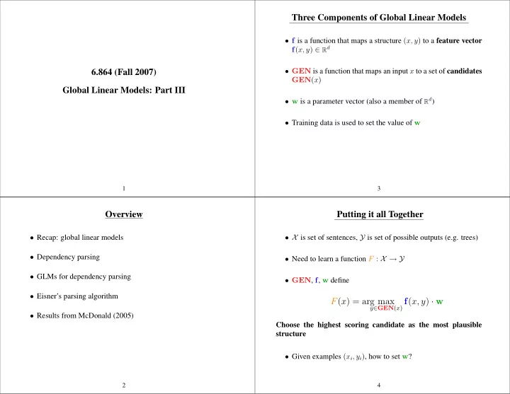
Three Components of Global Linear Models • f is a function that maps a structure ( x, y ) to a feature vector f ( x, y ) ∈ R d • GEN is a function that maps an input x to a set of candidates 6.864 (Fall 2007) GEN ( x ) Global Linear Models: Part III • w is a parameter vector (also a member of R d ) • Training data is used to set the value of w 1 3 Overview Putting it all Together • Recap: global linear models • X is set of sentences, Y is set of possible outputs (e.g. trees) • Dependency parsing • Need to learn a function F : X → Y • GLMs for dependency parsing • GEN , f , w define • Eisner’s parsing algorithm F ( x ) = arg max y ∈ GEN ( x ) f ( x, y ) · w • Results from McDonald (2005) Choose the highest scoring candidate as the most plausible structure • Given examples ( x i , y i ) , how to set w ? 2 4

She announced a program to promote safety in trucks and vans A tagged sentence with n words has n history/tag pairs ⇓ GEN Hispaniola/NNP quickly/RB became/VB an/DT important/JJ base/NN S S S S S S NP VP NP VP NP VP NP VP She She She NP VP NP VP She announced NP She announced NP She announced NP announced NP NP VP NP VP a program announced NP NP VP a program announced NP NP PP to promote NP a program to promote NP PP in NP safety NP VP safety PP in NP a program to promote trucks and vans in NP NP to promote NP trucks and vans safety trucks and vans NP and NP NP and NP vans vans NP and NP safety vans NP VP NP VP PP a program a program in NP to promote NP PP to promote NP trucks safety in NP History Tag safety PP trucks in NP trucks t − 2 t − 1 w [1: n ] i t ⇓ f ⇓ f ⇓ f ⇓ f ⇓ f ⇓ f � Hispaniola, quickly, . . . , � 1 NNP * * NNP � Hispaniola, quickly, . . . , � 2 RB * � 1 , 1 , 3 , 5 � � 2 , 0 , 0 , 5 � � 1 , 0 , 1 , 5 � � 0 , 0 , 3 , 0 � � 0 , 1 , 0 , 5 � � 0 , 0 , 1 , 5 � NNP RB � Hispaniola, quickly, . . . , � 3 VB RB VB � Hispaniola, quickly, . . . , � 4 DT ⇓ f · w ⇓ f · w ⇓ f · w ⇓ f · w ⇓ f · w ⇓ f · w VP DT � Hispaniola, quickly, . . . , � 5 JJ 13.6 12.2 12.1 3.3 9.4 11.1 DT JJ � Hispaniola, quickly, . . . , � 6 NN ⇓ arg max Define global features through local features: S NP VP n She announced NP � NP VP f ( t [1: n ] , w [1: n ] ) = g ( h i , t i ) a program to VP promote NP safety PP i =1 in NP NP and NP trucks vans where t i is the i ’th tag, h i is the i ’th history 5 7 A Variant of the Perceptron Algorithm Global and Local Features Inputs: Training set ( x i , y i ) for i = 1 . . . n • Typically, local features are indicator functions, e.g., Initialization: w = 0 � 1 if current word w i ends in ing and t = VBG F ( x ) = argmax y ∈ GEN ( x ) f ( x, y ) · w Define: g 101 ( h, t ) = 0 otherwise For t = 1 . . . T , i = 1 . . . n Algorithm: z i = F ( x i ) • and global features are then counts, If ( z i � = y i ) w = w + f ( x i , y i ) − f ( x i , z i ) f 101 ( w [1: n ] , t [1: n ] ) = Number of times a word ending in ing is Output: Parameters w tagged as VBG in ( w [1: n ] , t [1: n ] ) 6 8

Putting it all Together Training a Tagger Using the Perceptron Algorithm Inputs: Training set ( w i [1: n i ] , t i [1: n i ] ) for i = 1 . . . n . • GEN ( w [1: n ] ) is the set of all tagged sequences of length n Initialization: w = 0 • GEN , f , w define Algorithm: For t = 1 . . . T, i = 1 . . . n F ( w [1: n ] ) = arg t [1: n ] ∈ GEN ( w [1: n ] ) w · f ( w [1: n ] , t [1: n ] ) max u [1: ni ] ∈T ni w · f ( w i z [1: n i ] = arg max [1: n i ] , u [1: n i ] ) n � = arg max g ( h i , t i ) t [1: n ] ∈ GEN ( w [1: n ] ) w · i =1 z [1: n i ] can be computed with the dynamic programming (Viterbi) algorithm n � = arg max w · g ( h i , t i ) If z [1: n i ] � = t i t [1: n ] ∈ GEN ( w [1: n ] ) [1: n i ] then i =1 • Some notes: f ( w i [1: n i ] , t i [1: n i ] ) − f ( w i w = w + [1: n i ] , z [1: n i ] ) – Score for a tagged sequence is a sum of local scores Output: Parameter vector w . – Dynamic programming can be used to fi nd the argmax ! (because history only considers the previous two tags) 9 11 A Variant of the Perceptron Algorithm Overview • Recap: global linear models Inputs: Training set ( x i , y i ) for i = 1 . . . n • Dependency parsing Initialization: w = 0 F ( x ) = argmax y ∈ GEN ( x ) f ( x, y ) · w Define: • GLMs for dependency parsing For t = 1 . . . T , i = 1 . . . n Algorithm: • Eisner’s parsing algorithm z i = F ( x i ) If ( z i � = y i ) w = w + f ( x i , y i ) − f ( x i , z i ) • Results from McDonald (2005) Output: Parameters w 10 12

Unlabeled Dependency Parses A More Complex Example root John saw a movie that he liked today John saw a movie root • root is a special root symbol • Each dependency is a pair ( h, m ) where h is the index of a head word, m is the index of a modifi er word. In the fi gures, we represent a dependency ( h, m ) by a directed edge from h to m . • Dependencies in the above example are (0 , 2) , (2 , 1) , (2 , 4) , and (4 , 3) . (We take 0 to be the root symbol.) 13 15 All Dependency Parses for John saw Mary Conditions on Dependency Structures John saw Mary root root John saw a movie that he liked today John saw Mary root • The dependency arcs form a directed tree , with the root root John saw Mary symbol at the root of the tree. (Definition: A directed tree rooted at root is a tree, where for root John saw Mary root John saw Mary every word w other than the root, there is a directed path from root to w .) • There are no “crossing dependencies”. Dependency structures with no crossing dependencies are sometimes referred to as projective structures. 14 16

S(told,V) Labeled Dependency Parses NP(Hillary,NNP) VP(told,VBD) NNP Hillary V(told,VBD) NP(Clinton,NNP) SBAR(that,COMP) VBD NNP • Similar to unlabeled structures, but each dependency is a triple ( h, m, l ) COMP S told Clinton where h is the index of a head word, m is the index of a modifi er word, that NP(she,PRP) VP(was,Vt) and l is a label. In the fi gures, we represent a dependency ( h, m, l ) by a PRP directed edge from h to m with a label l . Vt NP(president,NN) she was NN • For most of this lecture we’ll stick to unlabeled dependency structures. president ( told VBD TOP S SPECIAL) (told VBD Hillary NNP S VP NP LEFT) (told VBD Clinton NNP VP VBD NP RIGHT) (told VBD that COMP VP VBD SBAR RIGHT) (that COMP was Vt SBAR COMP S RIGHT) (was Vt she PRP S VP NP LEFT) (was Vt president NP VP Vt NP RIGHT) 17 19 S(told,V) Extracting Dependency Parses from Treebanks • There’s recently been a lot of interest in dependency parsing. For example, NP(Hillary,NNP) VP(told,VBD) the CoNLL 2006 conference had a “shared task” where 12 languages NNP were involved (Arabic, Chinese, Czech, Danish, Dutch, German, Japanese, Hillary Portuguese, Slovene, Spanish, Swedish, Turkish). 19 different groups V(told,VBD) NP(Clinton,NNP) SBAR(that,COMP) developed dependency parsing systems. CoNLL 2007 had a similar shared VBD NNP task. Google for “conll 2006 shared task” for more details. For a recent COMP S told Clinton PhD thesis on the topic, see Ryan McDonald, Discriminative Training that NP(she,PRP) VP(was,Vt) and Spanning Tree Algorithms for Dependency Parsing , University of PRP Pennsylvania. Vt NP(president,NN) she was NN president • For some languages, e.g., Czech, there are “dependency banks” available Unlabeled Dependencies: which contain training data in the form of sentences paired with (for root → told) (0,2) dependency structures (for told → Hillary) (2,1) (for told → Clinton) (2,3) (for told → that) (2,4) • For other languages, we have treebanks from which we can extract (for that → was) (4,6) dependency structures, using lexicalized grammars described earlier in the (for was → she) (6,5) course (see Parsing and Syntax 2 ) (for was → president) (6,7) 18 20

Effi ciency of Dependency Parsing GLMs for Dependency parsing • PCFG parsing is O ( n 3 G 3 ) where n is the length of the • x is a sentence sentence, G is the number of non-terminals in the grammar • GEN ( x ) is set of all dependency structures for x • Lexicalized PCFG parsing is O ( n 5 G 3 ) where n is the length of the sentence, G is the number of non-terminals in the • f ( x, y ) is a feature vector for a sentence x paired with a grammar. (With the algorithms we’ve seen—it is possible to dependency parse y do a little better than this.) • Unlabeled dependency parsing is O ( n 3 ) . (See part 4 of these slides for the algorithm.) 21 23 Overview GLMs for Dependency parsing • To run the perceptron algorithm, we must be able to efficiently • Recap: global linear models calculate arg y ∈ GEN ( x ) w · f ( x, y ) max • Dependency parsing • Local feature vectors: define • Global Linear Models (GLMs) for dependency parsing � f ( x, y ) = g ( x, h, m ) • Eisner’s parsing algorithm ( h,m ) ∈ y where g ( x, h, m ) maps a sentence x and a dependency ( h, m ) • Results from McDonald (2005) to a local feature vector • Can then efficiently calculate � arg y ∈ GEN ( x ) w · f ( x, y ) = arg max max w · g ( x, h, m ) y ∈ GEN ( x ) ( h,m ) ∈ y 22 24