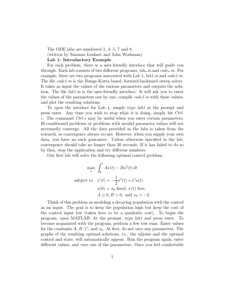
The ODE labs are numbered 1, 4, 5, 7 and 8. (written by Suzanne - PDF document

The ODE labs are numbered 1, 4, 5, 7 and 8. (written by Suzanne Lenhart and John Workman) Lab 1: Introductory Example For each problem, there is a user-friendly interface that will guide you through. Each lab consists of two different programs, lab .m and code .m . For example, there are two programs associated with Lab 1, lab1.m and code1.m . The file code1.m is the Runge-Kutta based, forward-backward sweep solver. It takes as input the values of the various parameters and outputs the solu- tion. The file lab1.m is the user-friendly interface. It will ask you to enter the values of the parameters one by one, compile code1.m with these values, and plot the resulting solutions. To open the interface for Lab 1, simply type lab1 at the prompt and press enter. Any time you wish to stop what it is doing, simply hit Ctrl- c . The command Ctrl-c may be useful when you enter certain parameters. Ill-conditioned problems or problems with invalid parameter values will not necessarily converge. All the data provided in the labs is taken from the research, so convergence always occurs. However, when you supply your own data, you have no such guarantee. Unless otherwise specified in the lab, convergence should take no longer than 30 seconds. If it has failed to do so by then, stop the application and try different numbers. Our first lab will solve the following optimal control problem. � 1 Ax ( t ) − Bu 2 ( t ) dt max u 0 x ′ ( t ) = − 1 2 x 2 ( t ) + Cu ( t ) subject to x (0) = x 0 fixed, x (1) free, A ≥ 0 , B > 0 , and x 0 > − 2 . Think of this problem as modeling a decaying population with the control as an input. The goal is to keep the population high but keep the cost of the control input low (taken here to be a quadratic cost). To begin the program, open MATLAB. At the prompt, type lab1 and press enter. To become acquainted with the program, perform a few test runs. Enter values for the constants A , B , C , and x 0 . At first, do not vary any parameters. The graphs of the resulting optimal solutions, i.e., the adjoint and the optimal control and state, will automatically appear. Run the program again, enter different values, and vary one of the parameters. Once you feel comfortable 1

with the structure of the program, begin working through the lab exercises below. This lab will focus on using the program to characterize the optimal control and resulting state and to ascertain how each parameter affects the solution. First, let us consider the goal of the problem. We want to use the control u to maximize the total value of x . However, we also want to maximize the negative squared value of u . This, of course, is equivalent to minimizing the squared value of u . Thus, we must find the right balance of increasing x and keeping u as small as possible. Enter the values A = B = x 0 = 1, C = 4 and do not vary any parameters, then look at the solutions. We see u begins strongly, pushing x up but steadily decreasing to 0. This makes logical sense when we consider the differential equation of x . Undisturbed by u , x will decrease monotonically. So, we want to push x up early, so that the natural decay will be less significant. As it is irrelevant when we use u , this is exactly what the optimal solution is. Also, note that x begins to decrease at the end of the interval, as the control approaches zero. Now try A = B = x 0 = 1, C = 4, and then vary the initial condition with x 0 = 2. As the second state begins higher, less control is needed to achieve a similar effect. Notice that the second control begins lower than the first, they quickly approach each other and are almost identical by t = 0 . 6. This causes the two states to move towards each other as well, although they never actually meet. Now use x 0 = − 1. This time, x begins below zero, so a greater control is needed to push the state up more quickly. Notice, however, we see the same effect as before, where the two controls eventually merge, although, much later than in the previous simulation. We mention here why the requirement x 0 > − 2 is imposed. If you were to solve the state equation without u (i.e., C = 0), you would find x 0 > − 2 is required, or division by 0 will occur and the state will blow-up in finite time. However, we know u will be used to increase x , so this condition is sufficient to give a finite state solution with the control. Use the values A = B = x 0 = 1, C = 4 varying C with C = 1. We have decreased the effect u has on the growth of the state. The optimal control in the second system is less than in the first. It is worth using a greater control in the first system, as it is more effective. Also, the second state, unlike the others we have seen, is decreasing over the whole interval. What little control is used does not increase the state, but only neutralizes some of the natural decay. It would now take far too much control to increase the state. Now, enter the same parameter values, this time varying with C = 8. 2

The results are as you might expect. The second optimal control, now more effective, is greater than than the first. The second state increases far more than the first, but still decreases as its control approaches zero. Finally, note that when C is varied, we do not have the two controls merging together. Enter A = B = x 0 = 1, C = 4 and vary with C = − 4. The control now has the opposite effect on the growth of the state. We see the control for the second state is merely the first control reflected across the x-axis, while the state and adjoint are the same. Try C = 0. Here, the control has no effect on x , so the optimal control is u ≡ 0, regardless of A , B , or x 0 . Re-enter the values A = B = x 0 = 1, C = 4. Choose to vary A . Specifically, try A = 4 as your second value. In the second system, A = 4 B , so maximizing x ( t ) is four times as important as minimizing u 2 ( t ). We see this playing out in the solutions. A greater u is used so that x can be increased appropriately. Conversely, enter A = B = x 0 = 1, C = 4 varying with B = 4. In this case, minimizing u 2 ( t ) is more important. We see on the graph, u ( t ) is pulled closer to zero, even though this causes x ( t ) to increase much less at the beginning. If you were to compare the graphs of the optimal solutions when A = 1, B = 2, for example, to the solutions when A = 2, B = 4, you would notice they were exactly the same. This is because the systems is only influenced by the ratio of the constants A and B , not the actual values. We know B � = 0, so we could divide it out of the integral. This would make our objective � 1 A B x ( t ) − u 2 ( t ) dt . Of course, the constant B in front of the function B 0 integral is irrelevant, so we ignore it. Thus, the only constant of significance in the integrand is A B . In all future labs, one term of the integrand will have no weight parameter, as it has been divided out. Before finishing, we look at a few special cases. Try A = 0. This will also cause the trivial solution u ∗ ≡ 0 regardless of B , C , and x 0 . If we no longer care about maximizing x , then we clearly should simply pick u ≡ 0 and ignore x . We cannot choose B = 0, because we divide by B in the optimality system. However, a similar situation occurs when B → 0. Try A = 1 and B = 0 . 01. Then, compare the graphs to A = 1 and B = 0 . 00001. A very large u (or large negative u , if C < 0) is used to push x up as quickly as possibly, because almost no importance is placed on keeping u 2 small. Lab 4: Introductory Example Continued: Bounded Case In this lab, we reexamine the first lab, this time imposing bounds on the control. Also notice that the weight parameter B has been removed from the 3