Survival Analysis Mark Lunt Centre for Epidemiology Versus - PowerPoint PPT Presentation
Introduction Censoring Describing Survival Comparing Survival Modelling Survival Survival Analysis Mark Lunt Centre for Epidemiology Versus Arthritis University of Manchester 22/12/2020 Introduction Censoring Describing Survival
Introduction Censoring Describing Survival Comparing Survival Modelling Survival Survival Analysis Mark Lunt Centre for Epidemiology Versus Arthritis University of Manchester 22/12/2020
Introduction Censoring Describing Survival Comparing Survival Modelling Survival Introduction Survival Analysis is concerned with the length of time before an event occurs. Initially, developed for events that can only occur once (e.g. death) Using time to event is more efficient that just whether or not the event has occured. It may be inconvenient to wait until the event occurs in all subjects. Need to include subjects whose time to event is not known (censored).
Introduction Censoring Describing Survival Comparing Survival Modelling Survival Plan of Talk Censoring Describing Survival Comparing Survival Modelling Survival
Introduction Censoring Describing Survival Comparing Survival Modelling Survival Censoring Exact time that event occured (or will occur) is unknown. Most commonly right-censored: we know the event has not occured yet. Maybe because the subject is lost to follow-up, or study is over. Makes no difference provided loss to follow-up is unrelated to outcome.
Introduction Censoring Describing Survival Comparing Survival Modelling Survival Censoring Examples: Chronological Time Time(months) 0 6 12 18 1 q ❛ 2 3 ❛ 4 ❛ 5 q 6 ❛ 7 q 8 ❛ 9 ❛ 10 q Patient Observation Accrual
Introduction Censoring Describing Survival Comparing Survival Modelling Survival Censoring Examples: Followup Time Time(months) 0 6 12 18 1 q 2 ❛ 3 ❛ 4 ❛ 5 q 6 ❛ 7 q 8 ❛ 9 ❛ 10 q Followup Time
Introduction Censoring Describing Survival Comparing Survival Modelling Survival Other types of censoring Left Censoring: Event had already occured before the study started. Subject cannot be included in study. May lead to bias. Interval Censoring: We know event occured between two fixed times, but not exactly when. E.g. Radiological damage: only picked up when film is taken.
Introduction Censoring Survivor function Describing Survival Stata Commands Comparing Survival Modelling Survival Describing Survival: Survival Curves Survivor function: S ( t ) probability of surviving to time t . If there are r k subjects at risk during the k th time-period, of whom f k fail, probability of surviving this time-period for those who reach it is r k − f k r k Probability of surviving the end of the k th time-period is the probability of surviving to the end of the ( k − 1 ) th time-period, times the probability of surviving the k th time-period. i.e S ( k ) = S ( k − 1 ) × r k − f k r k
Introduction Censoring Survivor function Describing Survival Stata Commands Comparing Survival Modelling Survival Motion Sickness Study 21 subjects put in a cabin on a hydraulic piston, Bounced up and down for 2 hours, or until they vomited, whichever occured first. Time to vomiting is our survival time. Two subjects insisted on ending the experiment early, although they had not vomited (censored). Is censoring independent of expected event time ? 14 subjects completed the 2 hours without vomiting. 5 subjects failed
Introduction Censoring Survivor function Describing Survival Stata Commands Comparing Survival Modelling Survival Motion Sickness Study Life-Table S ( t ) ID Time Censored r k f k 20 / 21 = 0 . 952 1 30 No 21 1 2 50 No 20 1 19 / 20 × S ( 30 ) = 0 . 905 3 50 Yes 19 0 19 / 19 × S ( 50 ) = 0 . 905 4 51 No 18 1 17 / 18 × S ( 50 ) = 0 . 855 5 66 Yes 17 0 17 / 17 × S ( 51 ) = 0 . 855 6 82 No 16 1 15 / 16 × S ( 66 ) = 0 . 801 7 92 No 15 1 14 / 15 × S ( 82 ) = 0 . 748 8 120 Yes 14 0 14 / 14 × S ( 92 ) = 0 . 748 . . . 21 120 Yes 14 0 14 / 14 × S ( 92 ) = 0 . 748
Introduction Censoring Survivor function Describing Survival Stata Commands Comparing Survival Modelling Survival Kaplan Meier Survival Curves Plot of S ( t ) against (t). Always start at (0, 1). Can only decrease. Drawn as a step function, with a downwards step at each failure time.
Introduction Censoring Survivor function Describing Survival Stata Commands Comparing Survival Modelling Survival Stata commands for Survival Analysis stset : sets data as survival Takes one variable: followup time Option failure = 1 if event occurred, 0 if censored sts list : produces life table sts graph : produces Kaplan Meier plot
Introduction Censoring Survivor function Describing Survival Stata Commands Comparing Survival Modelling Survival Stata Output sts list if group == 1 failure _d: fail analysis time _t: time Beg. Net Survivor Std. Time Total Fail Lost Function Error [95% Conf. Int.] ------------------------------------------------------------------------------- 30 21 1 0 0.9524 0.0465 0.7072 0.9932 50 20 1 1 0.9048 0.0641 0.6700 0.9753 51 18 1 0 0.8545 0.0778 0.6133 0.9507 66 17 0 1 0.8545 0.0778 0.6133 0.9507 82 16 1 0 0.8011 0.0894 0.5519 0.9206 92 15 1 0 0.7477 0.0981 0.4946 0.8868 120 14 0 14 0.7477 0.0981 0.4946 0.8868 -------------------------------------------------------------------------------
Introduction Censoring Survivor function Describing Survival Stata Commands Comparing Survival Modelling Survival Kaplan Meier Curve: example Kaplan−Meier survival estimate 1.00 0.75 0.50 0.25 0.00 0 50 100 150 analysis time
Introduction Censoring Describing Survival Comparing Survival Modelling Survival Comparing Survivor Functions Null Hypothesis Survival in both groups is the same Alternative Hypothesis Groups are different 1 One group is consistently better 2 One group is better at fixed time t 3 Groups are the same until time t , one group is better after 4 One group is worse up to time t , better afterwards. 5 No test is equally powerful against all alternatives.
Introduction Censoring Describing Survival Comparing Survival Modelling Survival Comparing Survivor Functions Can use Logrank test Most powerful against consistent difference Modified Wilcoxon Test Most powerful against early differences Regression Should decide which one to use beforehand.
Introduction Censoring Describing Survival Comparing Survival Modelling Survival Motion Sickness Revisited Less than 1/3 of subjects experienced an endpoint in first study. Further 28 subjects recruited Freqency and amplitude of vibration both doubled Intention was to induce vomiting sooner Were they successful ?
Introduction Censoring Describing Survival Comparing Survival Modelling Survival Comparing Survival Curves Kaplan−Meier survival estimates, by group 1.00 0.75 0.50 0.25 0.00 0 50 100 150 analysis time group = 1 group = 2
Introduction Censoring Describing Survival Comparing Survival Modelling Survival Comparison of Survivor Functions sts test group gives logrank test for differences between groups sts test group, wilcoxon gives Wilcoxon test χ 2 Test p Logrank 3.21 0.073 Wilcoxon 3.18 0.075
Introduction Censoring Describing Survival Comparing Survival Modelling Survival What to avoid Compare mean survival in each group. Censoring makes this meaningless Overinterpret the tail of a survival curve. There are generally few subjects in tails Compare proportion surviving in each group at a fixed time. Depends on arbitrary choice of time Lacks power compared to survival analysis Fine for description, not for hypothesis testing
Introduction The hazard function Censoring Cox Regression Describing Survival Proportional Hazards Assumption Comparing Survival Modelling Survival Modelling Survival Cannot often simply compare groups, must adjust for other prognostic factors. Predicting survival function S is tricky. Easier to predict the hazard function. Hazard function h ( t ) is the risk of dying at time t , given that you’ve survived until then. Can be calculated from the survival function. Survival function can be calculated from the hazard function. Hazard function easier to model
Introduction The hazard function Censoring Cox Regression Describing Survival Proportional Hazards Assumption Comparing Survival Modelling Survival The Hazard Function Hazard for all cause mortality for time since birth
Introduction The hazard function Censoring Cox Regression Describing Survival Proportional Hazards Assumption Comparing Survival Modelling Survival Options for Modelling Hazard Function Parametric Model Semi-parametric models Cox Regression (unrestricted baseline hazard) Smoothed baseline hazard
Introduction The hazard function Censoring Cox Regression Describing Survival Proportional Hazards Assumption Comparing Survival Modelling Survival Comparing Hazard Functions Exponential Distribution Log−Logistic Distribution 5 5 4 4 3 3 2 2 1 1 0 0 0 .5 1 1.5 2 0 .5 1 1.5 2 time time Untreated Treated Untreated Treated Unknown Baseline Hazard Non−constant Hazard Ratio 5 5 4 4 3 3 2 2 1 1 0 0 0 .5 1 1.5 2 0 .5 1 1.5 2 time time Untreated Treated Untreated Treated
Recommend
More recommend
Explore More Topics
Stay informed with curated content and fresh updates.
