Lecture 17: Survival Analysis -- Cox proportional Hazards Ani - PowerPoint PPT Presentation
Lecture 17: Survival Analysis -- Cox proportional Hazards Ani Manichaikul amanicha@jhsph.edu 14 May 2007 1 Survival Analysis n Suppose we have designed a study to estimate survival after chemotherapy treatment for patients with a certain
Lecture 17: Survival Analysis -- Cox proportional Hazards Ani Manichaikul amanicha@jhsph.edu 14 May 2007 1
Survival Analysis n Suppose we have designed a study to estimate survival after chemotherapy treatment for patients with a certain cancer n Patients received chemotherapy between 1990 and 1994 and were followed until death or the year 2000, whichever occurred first 2
Survival Analysis n In this study the event of interest is death n The time clock starts as soon as the subject finishes his/her chemotherapy treatments 3
Survival Analysis Dies 1990 1995 2000 4
Survival Analysis Dies Patient one enters in 1990, dies in 1995: Patient one survives five years 1990 1995 2000 5
Survival Analysis Lost to Follow-up 1990 1995 2000 6
Survival Analysis Lost to Follow-up Patient two enters in 1991, drops out in 1997: Patient two is lost to follow-up after six years 1990 1995 2000 7
Survival Analysis Withdrawn Alive (Administratively Censored) 1990 1995 2000 8
Survival Analysis Withdrawn Alive Patient three enters in 1993, is still alive at end of study: Patient three is still alive after seven years 1990 1995 2000 9
Survival Analysis n Patient: → 1995 5 years n 1: 1990 → 1997 6+ years n 2: 1991 → 2000 7+ years n 3: 1993 n Patients two and three are called censored observations 10
Central Problem n Estimation of the survival curve n S(t) = Proportion surviving at least to time t or beyond 11
Approaches n Life table method n Grouped in intervals n Kaplan-Meier (1958) n Ungrouped data n Small samples 12
Kaplan-Meier Estimate n Curve can be estimated at each event, but not at censoring times − ( ) ( ) n t y t = × S ( ) (Pr _ _ ) S t evious Event Time ( ) n t n y( t ) = # events at time t n n( t ) = # subjects at risk for event at time t 13
Kaplan-Meier Estimate n Curve can be estimated at each event, but not at censoring times − ( ) ( ) n t y t = × S ( ) (Pr _ _ ) S t evious Event Time ( ) n t Proportion of original sample making it to time t 14
Kaplan-Meier Estimate n Curve can be estimated at each event, but not at censoring times − ( ) ( ) n t y t = × S ( ) (Pr _ _ ) S t evious Event Time ( ) n t Proportion surviving to time t who survive beyond time t 15
Kaplan-Meier Estimate n Start estimate at first event time n No Chemotherapy Group: Time = 5 − − ( 5 ) ( 5 ) 12 2 10 n y = = = = ( 5 ) . 833 S n ( 5 ) 12 12 16
Kaplan-Meier Estimate n No Chemotherapy group: Time= 8 n 2 nd event time − − ( 8 ) ( 8 ) 10 2 n y = × = × S ( 8 ) S ( 5 ) (. 833 ) n ( 8 ) 10 8 = × = . 833 . 666 10 17
Kaplan-Meier Estimate n Skip over censoring times: Remove from number at risk for next event time n Continue through final event time 18
19
20
Kaplan-Meier Estimate n Graph is a step function n “Jumps” at each observed event time n Nothing is assumed about curved shape between each observed event time 21
Kaplan-Meier Estimate 22
Confidence Interval for S(t) Greenwood’s Formula Complementary log-log transformation 23
Greenwood’s Formula n Variance of S(t) y ∑ = ˆ ˆ j 2 ( ) [ ( )] ( ) Var S t S t − n n y ≤ j : t t j j j j n Standard Error t = ˆ SE GW ( ) [ ( )] Var S t 24
95% Confidence Interval n Using Greenwood’s formula, and approximate 95% CI for S(t) is ± ˆ ( ) 1 . 96 * SE ( ) S t GW t n There is a “problem”: the 95% Confidence Interval is not constrained to lie within the interval (0,1) 25
Alternative Confidence Interval n Complementary log-log transformation υ = − ˆ ˆ ( ) log[ log ( )] t S t n Variance of CLL: y ∑ j ( ) − n n y ≤ υ = j : t t j j j ˆ j Var[ ( ( t )] 2 y ∑ ( j ) log − n n y ≤ j : t t j j j j = υ ˆ SE CLL (t) Var[ ( ( t )] 26
95% CI based on complementary log-log transformation n Use CLL to obtain 95% confidence interval on S(t) ν υ t ± n Get 95% CI for : ( t ) ˆ ( ) 1 . 96 * SE CLL t ( ) 27
n Transform back to get 95% for S(t): Use the inverse transformation ( ) ν = (t) -e ( ) e S t to get the 95% CI for S(t): ( ) ( ) υ + υ − ˆ ˆ ( t ) 1 . 96 * SE ( t ) ( t ) 1 . 96 * SE ( t ) CLL CLL -e -e [ e , e ] ( ) ± = 1 . 96 * SE ( t ) ˆ CLL e [ S ( t )] 28
Back to the AML Data 29
Kaplan-Meier Estimates 30
95% CI: Greenwood n Var Greenwood �� (13)] = 0.818 2 1 1 + 11 * 10 10 * 9 = (0.116) 2 ± n 95% CI Greenwood = .818 1.96* (.116) = (.586, 1.05) 1.05 is out of Range! 31
Better 95% CI CLL transformation υ = − = − ˆ ˆ ( ) log[ log ( )] 1 . 605 t S t n 1 1 + 110 90 υ = ˆ Var[ ( ( 13 )] n 2 10 9 + log log 11 10 . 0202 = = . 502 . 04027 = ( 13 ) . 708 SE CLL 32
Better 95% CI CLL transformation n 95% CLL for S(13) [ ] ± 1 . 96 * (. 708 ) = e . 818 = (. 437 ,. 952 ) Does not contain 1! 33
95% CI for S(t) in the maintained on chemotherapy group 34
95% CI for S(t) in the not maintained on chemo group 35
Regression in Survival Analysis n The Kaplan-Meier estimate and log-rank tests are great ways to compare survival between groups without making too many assumptions. n But…we also want a simple summary measure that compares groups Solution: Regression Analysis 36
Regression in Survival Analysis n The regression model for the hazard function (instantaneous incidence rate) as a function of p explanatory X variables is specified as: λ = λ + β + β + + β n log hazard: log ( ; ) log ( ) ... t X t X X p X 0 1 1 2 2 p ) ( ) ( )( β β β λ = λ n hazard: X X X ( ; ) ( ) ... p p t X t e e e 1 1 2 2 0 ( ) β = λ X ( t ) e (Vector of X’s) 0 37
Interpretations n � 0 (t): Hazard (incidence) rate as a function of time when all X’s are zero often must center Xs to make � 0 (t) n interpretable n exp{ � 1 } : the relative hazard associated with a 1 unit change in X 1 (i.e., X 1 + 1 - vs- X 1 ), holding other Xs constant, independent of time 38
Interpretations: Relative Risk n exp{ � 1 } : the relative risk for X 1 + 1 -vs- X 1 , holding other Xs constant, independent of time n Other � s have similar interpretations 39
Interpretations n e �� : “multiplies” the baseline hazard � 0 (t) by the same amount regardless of the time t. n This is therefore a “proportional hazards” model n the effect of any (fixed) X is the same at any time during follow-up 40
Note n � is the focus whereas � 0 (t) is a nuisance variable n David Cox (1972) showed how to estimate � without having to assume a model for � 0 (t) n “Semi-parametric” n � 0 (t) is the baseline hazard n “non-parametric part of the model n �� are the regression coefficients n “parametric” part of the model 41
Why Cox Proportional Hazards Model is Different? n It uses the partial likelihood, not the likelihood n We do not assume a particular distribution for the failure time; we only assume proportional hazards 42
Results from AML Data n Semi-parametric model for the hazard (incidence) rate for the AML data β λ = λ X ( ) ( ) t t e i i 0 n Where n � i (t) is the hazard for person i at week t n � 0 (t) is the hazard if X i = 0 (not maintained group), and is the multiplicative effect of X i = 1 (maintained group) 43
Results from AML Data: n e -0.812 = 0.44: relative rate of AML relapse maintained vs not maintained n 1/.44 = 2.25 relative rate of AML relapse not-maintained vs maintained n 95% CI: [e -.812-1.96* .521 , e -.812+ 1.96* .521 ] n (1.22, 6.25) 44
Example: CABG surgery Cox model to compare two treatments, controlling for n several predictors (Fisher and Van Belle, 1993) Compare surgical (CABG) with medical treatment for n left main coronary heart disease Use mortality (time to death) as the response n variable Control for 7 risk factors (age at baseline and 6 n coronary status measures) in making the comparison Time variable is time from treatment initiation to n death or censoring due to the end of the study or lost to follow-up 45
Variables 46
Cox PH: CABG Surgery n Model for the log hazard rate (incidence of death): λ = λ + β + β + + β log ( t ; X ) log ( t ) X X ... X 0 1 2 2 8 8 n Model for the hazard rate ( ) β + β + + β λ = λ X X ... X ( ; ) 0 ) ( t X t e 1 1 2 2 8 8 47
Cox Model Results 48
Recommend
More recommend
Explore More Topics
Stay informed with curated content and fresh updates.
