Parametric Survival Analysis So far, we have focused primarily on - PowerPoint PPT Presentation

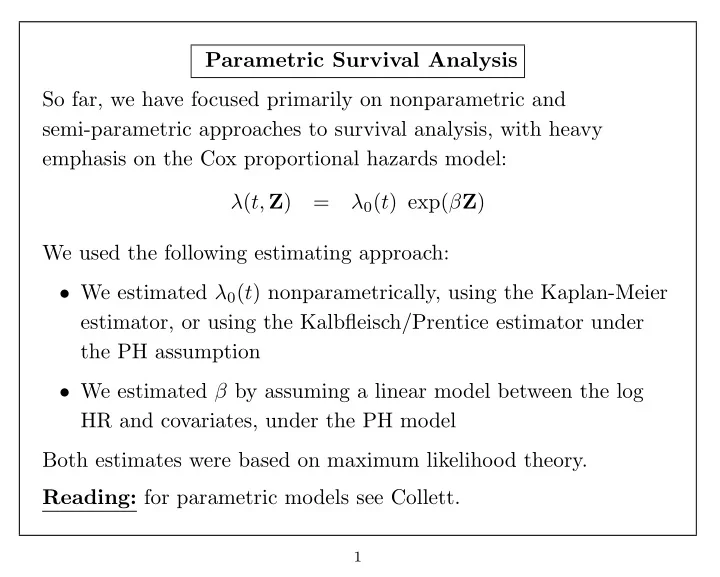
Parametric Survival Analysis So far, we have focused primarily on nonparametric and semi-parametric approaches to survival analysis, with heavy emphasis on the Cox proportional hazards model: λ ( t, Z ) = λ 0 ( t ) exp( β Z ) We used the following estimating approach: • We estimated λ 0 ( t ) nonparametrically, using the Kaplan-Meier estimator, or using the Kalbfleisch/Prentice estimator under the PH assumption • We estimated β by assuming a linear model between the log HR and covariates, under the PH model Both estimates were based on maximum likelihood theory. Reading: for parametric models see Collett. 1

There are several reasons why we should consider some alternative approaches based on parametric models: • The assumption of proportional hazards might not be appropriate (based on major departures) • If a parametric model actually holds, then we would probably gain efficiency • We may want to handle non-standard situations like – interval censoring – incorporating population mortality • We may want to make some connections with other familiar approaches (e.g. use of the Poisson likelihood) • We may want to obtain some estimates for use in designing a future survival study. 2

A simple start: Exponential Regression • Observed data: ( X i , δ i , Z i ) for individual i , Z i = ( Z i 1 , Z i 2 , ..., Z ip ) represents a set of p covariates. • Right censoring: Assume that X i = min( T i , U i ) • Survival distribution: Assume T i follows an exponential distribution with a parameter λ that depends on Z i , say λ i = Ψ( Z i ). Then we can write: T i ∼ exponential (Ψ( Z i )) 3

First, let’s review some facts about the exponential distribution (from our first survival lecture): λe − λt f ( t ) = for t ≥ 0 ∫ ∞ f ( u ) du = e − λt S ( t ) = P ( T ≥ t ) = t P ( T < t ) = 1 − e − λt F ( t ) = f ( t ) λ ( t ) = S ( t ) = λ constant hazard! ∫ t ∫ t Λ( t ) = λ ( u ) du = λ du = λt 0 0 4

Now, we say that λ is a constant over time t , but we want to let it depend on the covariate values, so we are setting λ i = Ψ( Z i ) The hazard rate would therefore be the same for any two individuals with the same covariate values. Although there are many possible choices for Ψ, one simple and natural choice is: Ψ( Z i ) = exp[ β 0 + Z i 1 β 1 + Z i 2 β 2 + ... + Z ip β p ] WHY? • ensures a positive hazard • for an individual with Z = 0 , the hazard is e β 0 . The model is called exponential regression because of the natural generalization from regular linear regression 5

Exponential regression for the 2-sample case: • Assume we have only a single covariate Z = Z , i.e., ( p = 1). Hazard Rate: Ψ( Z i ) = exp( β 0 + Z i β 1 ) Z i = 0 if individual i is in group 0 • Define: Z i = 1 if individual i is in group 1 • What is the hazard for group 0? • What is the hazard for group 1? • What is the hazard ratio of group 1 to group 0? • What is the interpretation of β 1 ? 6

Likelihood for Exponential Model Under the assumption of right censored data, each person has one of two possible contributions to the likelihood: (a) they have an event at X i ( δ i = 1) ⇒ contribution is � = e − λX i λ L i = S ( X i ) λ ( X i ) � · � �� � �� survive to X i fail at X i (b) they are censored at X i ( δ i = 0) ⇒ contribution is � = e − λX i L i = S ( X i ) � �� survive to X i 7

The likelihood is the product over all of the individuals: ∏ = L i L i ∏ ( λe − λX i ) δ i ( e − λX i ) (1 − δ i ) = � �� � � �� � i events censorings ∏ λ δ i ( e − λX i ) = i 8

Maximum Likelihood for Exponential How do we use the likelihood? • first take the log • then take the partial derivative with respect to β • then set to zero and solve for � β • this gives us the maximum likelihood estimators 9

The log-likelihood is: [∏ ] ( e − λX i ) λ δ i log L = log i ∑ = [ δ i log( λ ) − λX i ] i ∑ ∑ = [ δ i log( λ )] − λX i i i For the case of exponential regression, we now substitute the hazard λ = Ψ( Z i ) in the above log-likelihood: ∑ ∑ log L = [ δ i log(Ψ( Z i ))] − Ψ( Z i ) X i (1) i i 10

General Form of Log-likelihood for Right Censored Data In general, whenever we have right censored data, the likelihood and corresponding log likelihood will have the following forms: ∏ [ λ i ( X i )] δ i S i ( X i ) = L i ∑ ∑ log L = [ δ i log ( λ i ( X i ))] − Λ i ( X i ) i i where • λ i ( X i ) is the hazard for the individual i who fails at X i • Λ i ( X i ) is the cumulative hazard for an individual at their failure or censoring time For example, see the derivation of the likelihood for a Cox model on p.11-18 of Lecture 4 notes. We started with the likelihood above, then substituted the specific forms for λ ( X i ) under the PH assumption. 11

Consider our model for the hazard rate: λ = Ψ( Z i ) = exp[ β 0 + Z i 1 β 1 + Z i 2 β 2 + ... + Z ip β p ] We can write this using vector notation, as follows: (1 , Z i 1 , ...Z ip ) T Let = Z i and β = ( β 0 , β 1 , ...β p ) (Since β 0 is the intercept (i.e., the log hazard rate for the baseline group), we put a “1” as the first term in the vector Z i .) Then, we can write the hazard as: Ψ( Z i ) = exp[ β Z i ] Now we can substitute Ψ( Z i ) = exp[ β Z i ] in the log-likelihood shown in (1): n n ∑ ∑ log L = δ i ( β Z i ) − X i exp( β Z i ) i =1 i =1 12

Score Equations Taking the derivative with respect to β 0 , the score equation is: n ∑ ∂ log L = [ δ i − X i exp( β Z i )] ∂β 0 i =1 For β k , k = 1 , ...p , the equations are: n ∑ ∂ log L = [ δ i Z ik − X i Z ik exp( β Z i )] ∂β k i =1 n ∑ = Z ik [ δ i − X i exp( β Z i )] i =1 To find the MLE’s, we set the above equations to 0 and solve (simultaneously). The equations above imply that the MLE’s are obtained by setting the weighted number of failures ( ∑ i Z ik δ i ) equal to the weighted cumulative hazard ( ∑ i Z ik Λ( X i )). 13

To find the variance of the MLE’s, we need to take the second derivatives: − ∂ 2 log L n ∑ = Z ik Z ij X i exp( β Z i ) ∂β k ∂β j i =1 Some algebra (see Cox and Oakes section 6.2) reveals that [ Z ( I − Π) Z T ] − 1 β ) = I ( β ) − 1 = V ar ( � where • Z = ( Z 1 , . . . , Z n ) is a ( p + 1) × n matrix ( p covariates plus the “1” for the intercept β 0 ) • Π = diag ( π 1 , . . . , π n ) (this means that Π is a diagonal matrix, with the terms π 1 , . . . , π n on the diagonal) 14

• π i is the probability that the i -th person is censored, so (1 − π i ) is the probability that they failed. • Note: The information I ( β ) (inverse of the variance) is proportional to the number of failures, not the sample size. This will be important when we talk about study design. 15

The Single Sample Problem ( Z i = 1 for everyone): First, what is the MLE of β 0 ? = ∑ n We set ∂ log L i =1 [ δ i − X i exp( β 0 Z i )] equal to 0 and solve: ∂β 0 n n ∑ ∑ δ i = [ X i exp( β 0 )] ⇒ i =1 i =1 n ∑ d = exp( β 0 ) X i i =1 d exp( � ∑ n β 0 ) = i =1 X i d ˆ λ = t where d is the total number of deaths (or events), and t = ∑ X i is the total person-time contributed by all individuals. 16

If d/t is the MLE for λ , what does this imply about the MLE of β 0 ? [ Z ( I − Π) Z T ] − 1 , Using the previous formula V ar (ˆ β ) = what is the variance of � β 0 ?: With some matrix algebra, you can show that it is: i =1 (1 − π i ) = 1 1 V ar ( � ∑ n β 0 ) = d 17

λ = e ˆ What about ˆ β 0 ? By the delta method, λ 2 V ar ( � V ar (ˆ ˆ λ ) = β 0 ) = ? 18

The Two-Sample Problem: Z i Subjects Events Follow-up t 0 = ∑ n 0 Group 0: Z i = 0 n 0 d 0 i =1 X i t 1 = ∑ n 1 Group 1: Z i = 1 n 1 d 1 i =1 X i 19

The log-likelihood: n n ∑ ∑ log L = δ i ( β 0 + β 1 Z i ) − X i exp( β 0 + β 1 Z i ) i =1 i =1 n ∑ so ∂ log L = [ δ i − X i exp( β 0 + β 1 Z i )] ∂β 0 i =1 ( d 0 + d 1 ) − ( t 0 e β 0 + t 1 e β 0 + β 1 ) = n ∑ ∂ log L = Z i [ δ i − X i exp( β 0 + β 1 Z i )] ∂β 1 i =1 d 1 − t 1 e β 0 + β 1 = 20

β 0 + ˆ ˆ β 1 =? ˆ This implies: λ 1 = e ˆ β 0 =? ˆ λ 0 = e ˆ β 0 = ? ˆ β 1 = ? 21

Important Result: The maximum likelihood estimates (MLE’s) of the hazard rates under the exponential model are the number of events divided by the person-years of follow-up! (this result will be relied on heavily when we discuss study design) 22

Exponential Regression: Means and Medians Mean Survival Time For the exponential distribution, E ( T ) = 1 /λ . • Control Group: 1 / ˆ λ 0 = 1 / exp(ˆ T 0 = β 0 ) • Treatment Group: 1 / ˆ λ 1 = 1 / exp(ˆ β 0 + ˆ T 1 = β 1 ) 23

Median Survival Time This is the value M at which S ( t ) = e − λt = 0 . 5, so M = median = − log(0 . 5) λ • Control Group: − log(0 . 5) = − log(0 . 5) ˆ M 0 = ˆ exp(ˆ λ 0 β 0 ) • Treatment Group: − log(0 . 5) − log(0 . 5) ˆ M 1 = = ˆ exp(ˆ β 0 + ˆ λ 1 β 1 ) 24

Exponential Regression: Variance Estimates and Test Statistics We can also calculate the variances of the MLE’s as simple functions of the number of failures: 1 var (ˆ β 0 ) = d 0 1 + 1 var (ˆ β 1 ) = d 0 d 1 25