CMSC427 Notes on piecewise parametric curves: Hermite, Catmull-Rom, - PDF document

CMSC427 Notes on piecewise parametric curves: Hermite, Catmull-Rom, and Bezier I. Parametric curves and surfaces Model shapes and behavior with parametric curves Have done lines, circles, cylinders, superellipses, and others But limitations – how can we model an arbitrary shape? A face, a mountain? II. Solution: Piecewise parametric curves Model arbitrary shapes with piecewise parametric curves Each piece locally approximates part of a complex shape III. Continuity: parametric and geometric How to join piecewise sections? How to keep the overall curve smooth? Continuity at joining points, or knots Ck continuity – continuity of parametric curve and derivatives C0 – matching position C1 – matching position and direction (tangent), and speed C2 – matching position, direction and curvature Given f, g adjacent piecewise curves, we have for derivative i that 𝑔 (#) 𝑢 & = 𝑕 (#) 𝑢 & at 𝑢 & in knot k Gk continuity – geometric continuity without respect to arc length G0 – matching position G1 – matching position and direction (tangent), not always speed G2 – matching position, direction and curvature Given f, g adjacent piecewise curves, we have for derivative i that 𝑔 (#) 𝑢 & = 𝑡𝑕 (#) 𝑢 & at 𝑢 & in knot k, eg, the derivatives are proportional IV. Linear, quadratic and cubic curves Options for piecewise curves are linear, quadratic, cubic and higher order curves • Piecewise linear approximation – commonly used • Quadratic curve – used, but hard to get C1 continuity at both ends • Cubic curve – has inflection point, so can switch direction and achieve C1/C2 Used in industrial design – generally smooth enough for perception Not smooth enough for all applications – motion control, other Conclusion: cubic curve is adequate for most purposes

V. How to specify curves: control points and interpolation Control point – data point that controls shape of curve Interpolation – curve goes through control point Approximation – curve goes close to, or is controlled by, control point Local vs. global control – Local control, only nearby points control shape Global control, all points control entire curve VI. First example: Hermite cubic curve (2D version) Given a parametric equation of (x,y) in t in [0,1] 𝑦 𝑢 = 𝑏𝑢 , + 𝑐𝑢 / + 𝑑𝑢 + 𝑒 𝑧 𝑢 = 𝑓𝑢 , + 𝑔𝑢 / + 𝑕𝑢 + ℎ P1 = (x1,y1) T1=<dx1,dy1> P0=(x0,y0) The resulting curve interpolates points P0, P1 and matches tangents T0, T1 T0=<dx0,dy0> Since x(t) and y(t) are independent, consider first x(t) and four parameters a, b, c and d. (Developments for y(t), and z(t), are similar.) We have the derivative: 𝑦′ 𝑢 = 3𝑏𝑢 / + 2𝑐𝑢 + 𝑑 And we have the following four constraints at t = 0 (at P0) and t = 1 (at P1): 𝑦 0 = 𝑒 𝑦′(0) = 𝑑 𝑦 1 = 𝑏 + 𝑐 + 𝑑 + 𝑒 𝑦′ 1 = 3𝑏 + 2𝑐 + 𝑑 If we substitute and solve for a, b, c and d we get this curve that satisfies the constraints. 𝑒 = 𝑦0 𝑑 = 𝑒𝑦0 𝑐 = −3𝑦0 + 3𝑦1 − 2𝑒𝑦0 − 𝑒𝑦1 𝑏 = 2𝑦0 − 2𝑦1 + 𝑒𝑦0 + 𝑒𝑦1 Call this Hermite version 1. There will be similar equations for y(t) and z(t). 𝑦 𝑢 = (2𝑦0 − 2𝑦1 + 𝑒𝑦0 + 𝑒𝑦1)𝑢 , + (−3𝑦0 + 3𝑦1 − 2𝑒𝑦0 − 𝑒𝑦1)𝑢 / + (𝑒𝑦0)𝑢 + 𝑦0

VII. Matrix form of curves The development of the Hermite curve equations is fine, but can be more efficiently (and effectively) given in matrix format. If we rewrite the four constraint equations in matrix format 𝑦 0 = 𝑒 𝑦′(0) = 𝑑 𝑦 1 = 𝑏 + 𝑐 + 𝑑 + 𝑒 𝑦′ 1 = 3𝑏 + 2𝑐 + 𝑑 we get 0 0 0 1 𝑏 𝑦0 1 1 𝑐 𝑦1 1 1 = 𝑑 0 0 1 0 𝑒𝑦0 𝑒 3 2 1 0 𝑒𝑦1 or 𝑁𝐵 = 𝐻 with M the matrix, A the parameter vector, and G the geometry vector. Solving we get 𝐵 = 𝑁 >? 𝐻 or the Hermite basis matrix 2 −2 𝑏 1 1 𝑦0 −3 3 𝑐 −2 −1 𝑦1 = 𝑑 0 0 1 0 𝑒𝑦0 𝑒 1 0 𝑒𝑦1 0 0 Call this Hermite version 2, matrix form. The basis matrix 𝑁 >? is a compact representation. IIX. Vector matrix form To make the matrix representation more compact we replace the scalar x0, x1, etc, with point and vectors P0 = <x0,y0,z0>, P1 = <x1,y1,z1>, T0=<dx0,dy0,dz0>, T1=<dx1,dy1,dz1>, to get: 𝒃 2 −2 1 1 𝑸𝟏 𝒄 −3 3 −2 −1 𝑸𝟐 = 𝒅 0 0 𝑼𝟏 1 0 𝒆 1 0 𝑼𝟐 0 0 Now we have a polynomial with vector coefficients. Call this Hermite version 3. 𝑄 𝑢 = 𝒃𝑢 , + 𝒄𝑢 / + 𝒅𝑢 + 𝒆

There’s one additional representation 2 −2 𝒃 1 1 𝑸𝟏 −3 3 𝒄 −2 −1 𝑸𝟐 𝑄 𝑢 = 𝑢 , 𝑢 / = 𝑢 , 𝑢 / 𝑢 1 𝑢 1 𝒅 0 0 1 0 𝑼𝟏 𝒆 1 0 0 0 𝑼𝟐 IX. Blending functions. A fourth version of the Hermite equation rewrites it in terms of blending functions that weights each of the data points. We take the first version 𝑦 𝑢 = (2𝑦0 − 2𝑦1 + 𝑒𝑦0 + 𝑒𝑦1)𝑢 , + (−3𝑦0 + 3𝑦1 − 2𝑒𝑦0 − 𝑒𝑦1)𝑢 / + (𝑒𝑦0)𝑢 + 𝑦0 and group the data terms 𝑦 𝑢 = 2𝑢 , − 3𝑢 / + 1 𝑦0 + −2𝑢 , + 3𝑢 / 𝑦1 + 𝑢 , − 2𝑢 / + 𝑢 𝑒𝑦0 + 𝑢 , − 𝑢 / 𝑒𝑦1 To get the four blending functions ℎ00(𝑢) = 2𝑢 , − 3𝑢 / + 1 ℎ01(𝑢) = −2𝑢 , + 3𝑢 / ℎ10(𝑢) = 𝑢 , − 2𝑢 / + 𝑢 ℎ00(𝑢) = 𝑢 , − 𝑢 / From Wikipedia, the four blending functions graph as below. These four functions sum to 1, so represent an affine combination. The way to look at this is, each of the curves weight the input data points, so the red curve (h00) represents the proportion of P0 that contributes to the output point.

X. Computing the tangents If we’re given four points, we can set up a matrix to compute the tangents from four original points. Assuming these are 𝑦 >? , 𝑦 J , 𝑦 ? , and 𝑦 / , we can define the matrix H that takes the original points into the point/tangent vector, as in 𝐻 = 𝐼𝑄 , where P is a vector of the original points. This can be inserted into the Hermite equation Given our final Hermite equation version 5, our final version: 𝑦 J 1 −1 𝑏 −1 1 𝑦 ? −1 1 𝑐 1 −1 𝑄 𝑢 = 𝑢 , 𝑢 / = 𝑢 , 𝑢 / 𝑢 1 𝑢 1 𝑑 𝑦 >? −1 1 0 0 𝑒 𝑦 / 1 0 0 0 IIX. Catmull-Rom splines If you build a Hermite curve from a polyline you can have a problem with C1 continuity, as the obvious way to define tangents from point to point is not symmetric. At one control point the left and right tangents would not be equal. At control point P3 in the diagram below the left and right tangents are computed from P2 and P4, respectively. P3 P5 P1 right left P4 P2 P0 Catmull-Rom curves use a symmetric definition of the tangent at a control point by defining the slope at point Pi as the difference between P(i+1) and P(i-1). P3 P5 P1 P4 P2 P0

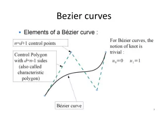
Our previous work with Hermite curves gives us most of the required math. The key is changing the tangent matrix H which computes derivatives at control points P0 and P1. (The ½ comes from weighting the tangent vector – we used a weight of 1 for Hermite curves, but it’s traditional to use ½ for Catmull-Rom. In the general development you’ll see a tuning factor of a .) 1 0 0 0 𝑦 J 𝑦0 0 1 0 0 𝑦 ? 𝑦1 = 𝑦 >? 1/2 0 −1/2 0 𝑒𝑦0′ 𝑦 / −1/2 0 0 1/2 𝑒𝑦1′ We use the same basis matrix as from the Hermite curves to get: or 𝑦 J 2 −2 𝑏 −0.5 0.5 𝑦 ? −3.5 3 𝑐 1 −0.5 𝑄 𝑢 = 𝑢 , 𝑢 / = 𝑢 , 𝑢 / 𝑢 1 𝑢 1 𝑑 𝑦 >? 0.5 0 0.5 0 𝑒 𝑦 / 1 0 0 0 XII. Bezier curves Finally, Bezier curves. These are often used graphics design, such as in programs like Adobe Illustrator. TrueType fonts use quadratic Bezier curves while Postscript and SVG use cubic. Bezier curves are deemed more flexible and intuitive, particularly for a sequence of points in a polyline, and can more easily manage kinks. The primary difference with Hermite is that the two middle points define the tangents, and the two end points are interpolated (in the four point version.) For an extended polyline a Bezier curve may not interpolated individual points beyond the first and final. The curve enters P0 on a tangent P0-P1, and exits P3 on a tangent P2-P3. The translate to our Hermite curve is given by:

P0 = P0 P1 = P3 T0 = 3(P1-P0) T1 = 3(P3-P2) The development of the Bezier curve can be done in the same fashion as Hermite from here. XIII. Defining Bezier curves with De Casteljau's algorithm See PowerPoint slides on this construction. Links http://graphics.stanford.edu/courses/cs148-09/lectures/splines.pdf https://pomax.github.io/bezierinfo/