CMSC427 Parametric curves: Hermite, Catmull-Rom, Bezier Modeling - PowerPoint PPT Presentation
CMSC427 Parametric curves: Hermite, Catmull-Rom, Bezier Modeling Creating 3D objects How to construct complicated surfaces? Goal Specify objects with few control points Resulting object should be visually pleasing (smooth)
CMSC427 Parametric curves: Hermite, Catmull-Rom, Bezier
Modeling • Creating 3D objects • How to construct complicated surfaces? • Goal • Specify objects with few control points • Resulting object should be visually pleasing (smooth) • Start with curves, then generalize to surfaces 2
Usefulness of curves • Surface of revolution 3
Usefulness of curves • Extruded/swept surfaces 4
Usefulness of curves • Animation • Provide a “track” for objects • Use as camera path 5
Usefulness of curves • Generalize to surface patches using “grids of curves”, next class 6
How to represent curves • Specify every point along curve? • Hard to get precise, smooth results • Too much data, too hard to work with • Idea: specify curves using small numbers of control points • Mathematics: use polynomials to represent curves Control point 7
Interpolating polynomial curves http://en.wikipedia.org/wiki/Polynomial_interpolation • Curve goes through all control points • Seems most intuitive • Surprisingly, not usually the best choice • Hard to predict behavior • Overshoots, wiggles • Hard to get “nice-looking” curves Control point Interpolating curve 8
Approximating polynomial curves • Curve is “influenced” by control points Control point • Various types & techniques based on polynomial functions • B é zier curves, B-splines, NURBS • Focus on B é zier curves 9
Mathematical definition • A vector valued function of one variable x ( t ) • Given t , compute a 3D point x =( x,y,z ) • May interpret as three functions x ( t ) , y ( t ), z( t ) • “Moving a point along the curve” x ( t ) z y x (0.0) x (0.5) x (1.0) x 10
Tangent vector • Derivative • A vector that points in the direction of movement • Length of x ’( t ) corresponds to speed x ( t ) z y x ’ (0.0) x ’ (0.5) x ’ (1.0) 11 x
Piecewise polynomial curves • Model complex shapes by sequence • Use polyline to store control points 12
Continuity • How piecewise curves join • Ck continuity – kth derivatives match • Gk continuity – kth derivatives are proportional 13
Hermite curves • Cubic curve (here 2D) 𝑦 𝑢 = 𝑏𝑢 3 + 𝑐𝑢 6 + 𝑑𝑢 + 𝑒 𝑧 𝑢 = 𝑓𝑢 3 + 𝑔𝑢 6 + 𝑢 + ℎ • Interpolates end points P0 and P1 • Matches tangent at endpoints T0 and T1 • (also dP0 and dP1 in these notes). P1 = (x1,y1) T1=<dx1,dy1> P0=(x0,y0) T0=<dx0,dy0>
Computing coefficients a, b, c and d • Derivative of x(t) 𝑦′ 𝑢 = 3𝑏𝑢 6 + 2𝑐𝑢 + 𝑑 • Set t = 0 and 1 for endpoints • Four constraints 𝑦 0 = 𝑒 𝑦′(0) = 𝑑 𝑦 1 = 𝑏 + 𝑐 + 𝑑 + 𝑒 𝑦′ 1 = 3𝑏 + 2𝑐 + 𝑑
Solve for a, b, c and d • Solve for a, b, c and d 𝑒 = 𝑦0 𝑑 = 𝑒𝑦0 𝑐 = −3𝑦0 + 3𝑦1 − 2𝑒𝑦0 − 𝑒𝑦1 𝑏 = 2𝑦0 − 2𝑦1 + 𝑒𝑦0 + 𝑒𝑦1
Matrix version • Constraints 𝑦 0 = 𝑒 𝑦′(0) = 𝑑 𝑦 1 = 𝑏 + 𝑐 + 𝑑 + 𝑒 𝑦′ 1 = 3𝑏 + 2𝑐 + 𝑑 • Give 0 0 0 1 𝑏 𝑦0 1 1 1 1 𝑐 𝑦1 = 𝑑 0 0 𝑒𝑦0 1 0 𝑒 3 2 𝑒𝑦1 1 0
Solve matrix version: basis matrix • Since we have 𝑁𝐵 = 𝐻 • We can solve with 𝐵 = 𝑁 \] 𝐻 • And get Hermite basis matrix 𝑁 \] 2 −2 𝑏 𝑦0 1 1 −3 3 𝑐 −2 −1 𝑦1 = 𝑑 0 0 𝑒𝑦0 1 0 𝑒 1 0 𝑒𝑦1 0 0
Vector version • To include x, y and z, rewrite with vectors P0, P1 and tangents T0 and T1 2 −2 𝒃 1 1 𝑸𝟏 −3 3 𝒄 −2 −1 𝑸𝟐 = 𝒅 0 0 𝑼𝟏 1 0 𝒆 1 0 𝑼𝟐 0 0 • Coefficients a, b, c and d are now vectors
Full polynomial version • Rewrite polynomial as dot product 𝒃 𝒄 𝑄 𝑢 = 𝑢 3 𝑢 6 𝑢 1 𝒅 𝒆 • 2 −2 1 1 𝑸𝟏 −3 3 −2 −1 𝑸𝟐 = 𝑢 3 𝑢 6 𝑢 1 0 0 𝑼𝟏 1 0 1 0 𝑼𝟐 0 0
Blending functions • Instead of polynomial in t, look at curve as weighted sum of P0, P1, T0 and T1 • 𝑦 𝑢 = 2𝑦0 − 2𝑦1 + 𝑒𝑦0 + 𝑒𝑦1 𝑢 3 • + −3𝑦0 + 3𝑦1 − 2𝑒𝑦0 − 𝑒𝑦1 𝑢 6 • + 𝑒𝑦0 𝑢 • +𝑦0
Blending functions • Instead of polynomial in t, look at curve as weighted sum of P0, P1, T0 and T1 • 𝑦 𝑢 = • 2𝑢 3 − 3𝑢 6 + 1 𝑦0 • + −2𝑢 3 + 3𝑢 6 𝑦1 • + 𝑢 3 − 2𝑢 6 + 𝑢 𝑒𝑦0 • + 𝑢 3 − 𝑢 6 𝑒𝑦1
Blending functions ℎ00(𝑢) = 2𝑢 3 − 3𝑢 6 + 1 ℎ01(𝑢) = −2𝑢 3 + 3𝑢 6 • ℎ10(𝑢) = 𝑢 3 − 2𝑢 6 + 𝑢 ℎ11(𝑢) = 𝑢 3 − 𝑢 6
Computing Hermite tangents • Have P(-1), P0, P1 and P2 as input • Compute tangent with H matrix 𝑦 o 1 0 𝑦0 0 0 𝑦 ] 0 1 𝑦1 0 0 = 𝑦 \] 𝑒𝑦0 −1 1 0 0 𝑦 6 0 0 𝑒𝑦1 −1 1
Combine with Hermite basis • Unify notation 𝑦 o 2 −2 1 0 𝑏 1 1 0 0 𝑦 ] −3 3 0 1 𝑐 −2 −1 0 0 = 𝑑 𝑦 \] 0 0 1 0 1 0 −1 0 𝑒 𝑦 6 1 0 0 −1 0 0 0 1 • Final matrix 𝑦 o 3 −3 𝑏 −1 1 𝑦 ] −5 4 𝑐 2 −1 = • 𝑑 𝑦 \] 1 0 −1 0 𝑒 𝑦 6 1 0 0 0
Catmull-Rom curves • Hermite – problem with C1 continuity P3 P5 P1 right left P4 P2 P0
Catmull-Rom curves • Catmull-Rom – make tangent symmetric • Define by two adjacent points • Here T3 = P4-P2 P3 P5 P1 P4 P2 P0
Catmull-Rom curves • Need to change H matrix • ½ traditional for C-R curves 1 0 𝑦 o 0 0 𝑦0 0 1 𝑦 ] 0 0 𝑦1 = 𝑦 \] −1/2 0 1/2 0 𝑒𝑦0′ 𝑦 6 0 1/2 −1/2 0 𝑒𝑦1′
Catmull-Rom curves • Which gives 1 0 𝑦 o 0 0 2 −2 𝑏 1 1 0 1 𝑦 ] 0 0 −3 3 𝑐 −2 −1 = 𝑑 𝑦 \] −1/2 0 1/2 0 0 0 1 0 𝑒 𝑦 6 0 1/2 1 0 −1/2 0 0 0 • Or 𝑦 o 2 −2 −0.5 0.5 𝑏 𝑦 ] −3.5 3 𝑐 1 −0.5 = 𝑑 𝑦 \] 0.5 0 0.5 0 𝑒 𝑦 6 1 0 0 0
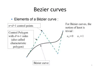
B é zier curves http://en.wikipedia.org/wiki/B%C3%A9zier_curve • A particularly intuitive way to define control points for polynomial curves • Developed for CAD (computer aided design) and manufacturing • Before games, before movies, CAD was the big application for CG • Pierre B é zier (1962), design of auto bodies for Peugeot, http://en.wikipedia.org/wiki/Pierre_B%C3%A9zier • Paul de Casteljau (1959), for Citroen 30
B é zier curves • Higher order extension of linear interpolation • Control points p 0 , p 1 , ... p 1 p 1 p 2 p 1 p 3 p 0 p 0 p 0 p 2 Linear Quadratic Cubic 31
B é zier curves • Intuitive control over curve given control points • Endpoints are interpolated, intermediate points are approximated • Convex Hull property • Variation-diminishing property 32
Cubic Bézier curve • Cubic polynomials, most common case • Defined by 4 control points • Two interpolated endpoints • Two midpoints control the tangent at the endpoints p 1 Control • polyline x ( t ) p 0 p 2 p 3 33
Bézier Curve formulation • Three alternatives, analogous to linear case 1. Weighted average of control points 2. Cubic polynomial function of t 3. Matrix form • Algorithmic construction • de Casteljau algorithm 34
de Casteljau Algorithm http://en.wikipedia.org/wiki/De_Casteljau's_algorithm • A recursive series of linear interpolations • Works for any order, not only cubic • Not terribly efficient to evaluate • Other forms more commonly used • Why study it? • Intuition about the geometry • Useful for subdivision (later today) 35
de Casteljau Algorithm • Given the control points • A value of t p 1 • Here t ≈ 0.25 p 0 p 2 p 3 36
de Casteljau Algorithm p 1 q 1 q 0 ( ) q 0 ( t ) = Lerp t , p 0 , p 1 p 0 p 2 ( ) q 1 ( t ) = Lerp t , p 1 , p 2 ( ) q 2 ( t ) = Lerp t , p 2 , p 3 q 2 p 3 37
de Casteljau Algorithm q 1 r 0 q 0 r 1 ( ) r 0 ( t ) = Lerp t , q 0 ( t ), q 1 ( t ) ( ) 1 ( t ) = Lerp t , q 1 ( t ), q 2 ( t ) r q 2 38
de Casteljau Algorithm r 0 • x r 1 ( ) x ( t ) = Lerp t , r 0 ( t ), r 1 ( t ) 39
de Casteljau algorithm p 1 • x p 0 p 2 • Applets p 3 • http://www2.mat.dtu.dk/people/J.Gravesen/cagd/decast.html • http://www.caffeineowl.com/graphics/2d/vectorial/bezierintro.html 40
de Casteljau Algorithm http://en.wikipedia.org/wiki/De_Casteljau's_algorithm Quadratic Linear Quartic Cubic 41
Recursive linear interpolation p 0 ( ) q 0 = Lerp t , p 0 , p 1 ( ) r 0 = Lerp t , q 0 , q 1 p 1 ( ) ( ) q 1 = Lerp t , p 1 , p 2 x = Lerp t , r 0 , r ( ) 1 1 = Lerp t , q 1 , q 2 p 2 r ( ) q 2 = Lerp t , p 2 , p 3 p 3 p 1 q 0 r 0 p 2 x q 1 r p 3 1 q 2 p 4 42
Recursive linear interpolation p 0 ( ) q 0 = Lerp t , p 0 , p 1 ( ) r 0 = Lerp t , q 0 , q 1 p 1 ( ) ( ) q 1 = Lerp t , p 1 , p 2 x = Lerp t , r 0 , r ( ) 1 1 = Lerp t , q 1 , q 2 p 2 r ( ) q 2 = Lerp t , p 2 , p 3 p 3 p 1 q 0 r 0 p 2 x q 1 r p 3 1 q 2 p 4 43
Recursive linear interpolation p 0 ( ) q 0 = Lerp t , p 0 , p 1 ( ) r 0 = Lerp t , q 0 , q 1 p 1 ( ) ( ) q 1 = Lerp t , p 1 , p 2 x = Lerp t , r 0 , r ( ) 1 1 = Lerp t , q 1 , q 2 p 2 r ( ) q 2 = Lerp t , p 2 , p 3 p 3 p 1 q 0 r 0 p 2 x q 1 r p 3 1 q 2 p 4 44
Recommend
More recommend
Explore More Topics
Stay informed with curated content and fresh updates.
