Survival analysis Niels Richard Hansen (Univ. Copenhagen) - PowerPoint PPT Presentation
Survival analysis Niels Richard Hansen (Univ. Copenhagen) Statistics BI/E lecture March 18, 2009 1 / 8 Survival analysis or reliability analysis, or simple point process models. The topic has its own development with focus on aspects of
Survival analysis Niels Richard Hansen (Univ. Copenhagen) Statistics BI/E lecture March 18, 2009 1 / 8
Survival analysis – or reliability analysis, or simple point process models. The topic has its own development with focus on aspects of models and distributions that differ from many other applications of statistics. This is primarily due to the following two issues: Niels Richard Hansen (Univ. Copenhagen) Statistics BI/E lecture March 18, 2009 1 / 8
Survival analysis – or reliability analysis, or simple point process models. The topic has its own development with focus on aspects of models and distributions that differ from many other applications of statistics. This is primarily due to the following two issues: Survival distributions are skewed distributions on the positive half line. It is the shape of the distribution rather than the location of the distribution that is of interest. Niels Richard Hansen (Univ. Copenhagen) Statistics BI/E lecture March 18, 2009 1 / 8
Survival analysis – or reliability analysis, or simple point process models. The topic has its own development with focus on aspects of models and distributions that differ from many other applications of statistics. This is primarily due to the following two issues: Survival distributions are skewed distributions on the positive half line. It is the shape of the distribution rather than the location of the distribution that is of interest. There is almost always a censoring mechanism, and certain aspects of the data are consequently missing. We need to deal with this in the modeling. Niels Richard Hansen (Univ. Copenhagen) Statistics BI/E lecture March 18, 2009 1 / 8
Example I In medicine we want to test whether a new, promising drug can prolong the life of humans. Niels Richard Hansen (Univ. Copenhagen) Statistics BI/E lecture March 18, 2009 2 / 8
Example I In medicine we want to test whether a new, promising drug can prolong the life of humans. We set up a controlled, double-blinded experiment with 1000 individuals of age 55 given this drug and a control group of 1000 individuals of age 55 given a placebo drug (disregarding any ethical considerations at this point). The test runs for 10 years, and approximately 10% of the participants in both groups abandon the experiment without dying – they are the censored observations. Niels Richard Hansen (Univ. Copenhagen) Statistics BI/E lecture March 18, 2009 2 / 8
Example I In medicine we want to test whether a new, promising drug can prolong the life of humans. We set up a controlled, double-blinded experiment with 1000 individuals of age 55 given this drug and a control group of 1000 individuals of age 55 given a placebo drug (disregarding any ethical considerations at this point). The test runs for 10 years, and approximately 10% of the participants in both groups abandon the experiment without dying – they are the censored observations. Those that survive for 10 years are all censored at that time - but this is less problematic. Niels Richard Hansen (Univ. Copenhagen) Statistics BI/E lecture March 18, 2009 2 / 8
Example II In engineering we want to estimate the life time of an electrical component. We record whenever a component is put to work and whenever a component fails. At any given time, all components in work that have not yet failed are censored. Niels Richard Hansen (Univ. Copenhagen) Statistics BI/E lecture March 18, 2009 3 / 8
Example II In engineering we want to estimate the life time of an electrical component. We record whenever a component is put to work and whenever a component fails. At any given time, all components in work that have not yet failed are censored. To estimate the life time based on the observed life times for the components that have failed up to this time will give a too pessimistic, biased result. Niels Richard Hansen (Univ. Copenhagen) Statistics BI/E lecture March 18, 2009 3 / 8
Example III A “real” survival application. Niels Richard Hansen (Univ. Copenhagen) Statistics BI/E lecture March 18, 2009 4 / 8
Example III A “real” survival application. Patients are enrolled in a study whenever they are diagnosed with a given (serious, life threatening) disease. Data on the subjects are collected – and may be collected regularly. Niels Richard Hansen (Univ. Copenhagen) Statistics BI/E lecture March 18, 2009 4 / 8
Example III A “real” survival application. Patients are enrolled in a study whenever they are diagnosed with a given (serious, life threatening) disease. Data on the subjects are collected – and may be collected regularly. At a planned calendar time the statistical analysis is done, and patients alive at this time are censored. Niels Richard Hansen (Univ. Copenhagen) Statistics BI/E lecture March 18, 2009 4 / 8
Example III A “real” survival application. Patients are enrolled in a study whenever they are diagnosed with a given (serious, life threatening) disease. Data on the subjects are collected – and may be collected regularly. At a planned calendar time the statistical analysis is done, and patients alive at this time are censored. Many questions are of interest, e.g. how different covariates affect the survival for this particular disease. One issue may be to compare the effect of two or more treatments on the survival. Niels Richard Hansen (Univ. Copenhagen) Statistics BI/E lecture March 18, 2009 4 / 8
The Kaplan-Meier estimator Based on the censored survival observations ( T i , ∆ i ) the Kaplan-Meier estimator is � 1 − ∆ N ( s ) � ˆ � S ( t ) = . Y ( s ) s ≤ t Niels Richard Hansen (Univ. Copenhagen) Statistics BI/E lecture March 18, 2009 5 / 8
The Kaplan-Meier estimator Based on the censored survival observations ( T i , ∆ i ) the Kaplan-Meier estimator is � 1 − ∆ N ( s ) � ˆ � S ( t ) = . Y ( s ) s ≤ t If τ i denotes the time for the i ’th jump � 1 � � 1 � � 1 � ˆ S ( t ) = 1 − 1 − . . . 1 − Y ( τ 1 ) Y ( τ 2 ) Y ( τ N ( t ) ) Niels Richard Hansen (Univ. Copenhagen) Statistics BI/E lecture March 18, 2009 5 / 8
The Kaplan-Meier estimator Based on the censored survival observations ( T i , ∆ i ) the Kaplan-Meier estimator is � 1 − ∆ N ( s ) � ˆ � S ( t ) = . Y ( s ) s ≤ t If τ i denotes the time for the i ’th jump � 1 � � 1 � � 1 � ˆ S ( t ) = 1 − 1 − . . . 1 − Y ( τ 1 ) Y ( τ 2 ) Y ( τ N ( t ) ) This estimator is the survival analysis version of the empirical distribution function. Niels Richard Hansen (Univ. Copenhagen) Statistics BI/E lecture March 18, 2009 5 / 8
The Cox proportional hazards model With covariates X i = ( X 1 i , . . . , X mi ) T the hazard rate for the i ’th individual is m � � � = α 0 ( t ) exp X T β α i ( t , X i ) = α 0 ( t ) exp β j X ij j =1 for an m -dimensional vector β of parameters. This is the Cox model. Niels Richard Hansen (Univ. Copenhagen) Statistics BI/E lecture March 18, 2009 6 / 8
The Cox proportional hazards model With covariates X i = ( X 1 i , . . . , X mi ) T the hazard rate for the i ’th individual is m � � � = α 0 ( t ) exp X T β α i ( t , X i ) = α 0 ( t ) exp β j X ij j =1 for an m -dimensional vector β of parameters. This is the Cox model. The parameters are estimated by solving the estimating equation n � ( X i − E ( β, T i ))∆ i = 0 i =1 where i 1( t ≤ T i ) X i exp( X T � i β ) E ( β, T i ) = i β ) . � i 1( t ≤ T i ) exp( X T Niels Richard Hansen (Univ. Copenhagen) Statistics BI/E lecture March 18, 2009 6 / 8
The Cox proportional hazards model With covariates X i = ( X 1 i , . . . , X mi ) T the hazard rate for the i ’th individual is m � � � = α 0 ( t ) exp X T β α i ( t , X i ) = α 0 ( t ) exp β j X ij j =1 for an m -dimensional vector β of parameters. This is the Cox model. The parameters are estimated by solving the estimating equation n � ( X i − E ( β, T i ))∆ i = 0 i =1 where i 1( t ≤ T i ) X i exp( X T � i β ) E ( β, T i ) = i β ) . � i 1( t ≤ T i ) exp( X T Detailed knowledge is available on the theoretical merits of this method. Niels Richard Hansen (Univ. Copenhagen) Statistics BI/E lecture March 18, 2009 6 / 8
Some further topics Diagnostic and residuals. To carry out a serious, practical analysis of survival data it is mandatory to take some steps to verify that the model actually fits the data, to check for outliers and/or highly influential observations. Several types of residuals can be introduced (cf. also generalized linear models), but no one general type of residuals and/or plots stand out clear (to me) as the winner. See Chapter 4 in Therneau and Grambsch . Niels Richard Hansen (Univ. Copenhagen) Statistics BI/E lecture March 18, 2009 7 / 8
Recommend
More recommend
Explore More Topics
Stay informed with curated content and fresh updates.
