Survival Analysis: Introduction Survival Analysis typically focuses - PowerPoint PPT Presentation
Survival Analysis: Introduction Survival Analysis typically focuses on time to event data. In the most general sense, it consists of techniques for positive-valued random variables, such as time to death time to onset (or relapse) of a
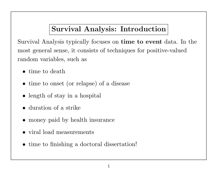
Survival Analysis: Introduction Survival Analysis typically focuses on time to event data. In the most general sense, it consists of techniques for positive-valued random variables, such as • time to death • time to onset (or relapse) of a disease • length of stay in a hospital • duration of a strike • money paid by health insurance • viral load measurements • time to finishing a doctoral dissertation! 1
Kinds of survival studies include: • clinical trials • prospective cohort studies • retrospective cohort studies Typically, survival data are not fully observed, but rather are censored . 2
In this course, we will: • describe survival data • compare survival of several groups • explain survival with covariates • design studies with survival endpoints 3
Some useful references: • Collett: Modelling Survival Data in Medical Research • Cox and Oakes: Analysis of Survival Data • Kleinbaum: Survival Analysis: A self-learning text • Klein & Moeschberger: Survival Analysis: Techniques for censored and truncated data • Cantor: Extending SAS Survival Analysis Techniques for Medical Research • Allison: Survival Analysis Using the SAS System 4
Some Definitions and notation Failure time random variables are always non-negative . That is, if we denote the failure time by T , then T ≥ 0. T can either be discrete (taking a finite set of values, e.g. a 1 , a 2 , . . . , a n ) or continuous (defined on (0 , ∞ )). A random variable X is called a censored failure time random variable if X = min( T, U ), where U is a non-negative censoring variable. 5
In order to define a failure time random variable, we need: (1) an unambiguous time origin (e.g. randomization to clinical trial, purchase of car) (2) a time scale (e.g. real time (days, years), mileage of a car) (3) definition of the event (e.g. death, need a new car transmission) 6
Illustration of survival data X t t X t X t study study opens closes = censored observation ② X = event 7
The illustration of survival data on the previous page shows several features which are typically encountered in analysis of survival data: • individuals do not all enter the study at the same time • when the study ends, some individuals still haven’t had the event yet • other individuals drop out or get lost in the middle of the study, and all we know about them is the last time they were still “free” of the event The first feature is referred to as “staggered entry” The last two features relate to “censoring” of the failure time events. 8
Types of censoring: • Right-censoring : only the r.v. X i = min( T i , U i ) is observed due to – loss to follow-up – drop-out – study termination We call this right-censoring because the true unobserved event is to the right of our censoring time; i.e., all we know is that the event has not happened at the end of follow-up. 9
In addition to observing X i , we also get to see the failure indicator : 1 if T i ≤ U i δ i = 0 if T i > U i Some software packages instead assume we have a censoring indicator : 0 if T i ≤ U i c i = 1 if T i > U i Right-censoring is the most common type of censoring assumption we will deal with in survival analysis. 10
• Left-censoring Can only observe Y i = max( T i , U i ) and the failure indicators: 1 if U i ≤ T i ǫ i = 0 if U i > T i e.g. In studies of time to HIV seroconversion, some of the enrolled subjects have already seroconverted at entry into the study - they are left-censored. 11
• Interval-censoring Observe ( L i , R i ) where T i ∈ ( L i , R i ) ex #1: Time to prostate cancer, observe longitudinal PSA measurements ex #2: Time to undetectable viral load in AIDS studies, based on measurements of viral load taken at each clinic visit 12
Independent versus informative censoring • We say censoring is independent (non-informative) if U i is independent of T i . – ex.1 If U i is the planned end of the study (say, 2 years after the study opens), then it is usually independent of the event times – ex.2 If U i is the time that a patient drops out of the study because they’ve gotten much sicker and/or had to discontinue taking the study treatment, then U i and T i are probably not independent 13
An individual censored at U should be representative of all subjects who survive to U . This means that censoring at U could depend on prognostic characteristics measured at baseline, but that among all those with the same baseline characteristics, the probability of censoring prior to or at time U should be the same. • Censoring is considered informative if the distribution of U i contains any information about the parameters characterizing the distribution of T i . 14
Suppose we have a sample of observations on n people: ( T 1 , U 1 ) , ( T 2 , U 2 ) , ..., ( T n , U n ) There are three main types of censoring times: • Type I: All the U i ’s are the same e.g. animal studies, all animals sacrificed after 2 years • Type II: U i = T ( r ) , the time of the r th failure. e.g. animal studies, stop when 4/6 have tumors • Random: the U i ’s are random variables, δ i ’s are failure indicators: 1 if T i ≤ U i δ i = 0 if T i > U i 15
Some example datasets: Example A. Duration of nursing home stay (Morris et al., Case Studies in Biometry , Ch 12) The National Center for Health Services Research studied 36 for-profit nursing homes to assess the effects of different financial incentives on length of stay. “Treated” nursing homes received higher per diems for Medicaid patients, and bonuses for improving a patient’s health and sending them home. Study included 1601 patients admitted between May 1, 1981 and April 30, 1982. 16
Variables include: LOS - Length of stay of a resident (in days) AGE - Age of a resident RX - Nursing home assignment (1:bonuses, 0:no bonuses) GENDER - Gender (1:male, 0:female) MARRIED - (1: married, 0:not married) HEALTH - health status (2:second best, 5:worst) FAIL - Failure/Censoring indicator (1:discharged,0:censored) First few lines of data: 37 86 1 0 0 2 0 61 77 1 0 0 4 0 17
Example B. Fecundability Women who had recently given birth were asked to recall how long it took them to become pregnant, and whether or not they smoked during that time. The outcome of interest is time to pregnancy (in menstrual cycles). Cycle Smokers Non-smokers 1 29 198 2 16 107 3 17 55 4 4 38 5 3 18 6 9 22 7 4 7 8 5 9 9 1 5 10 1 3 11 1 6 12 3 6 12+ 7 12 18
Example C: MAC Prevention Clinical Trial ACTG 196 was a randomized clinical trial to study the effects of combination regimens on prevention of MAC ( mycobacterium avium complex ), one of the most common OIs in AIDS patients. The treatment regimens were: • clarithromycin (new) • rifabutin (standard) • clarithromycin plus rifabutin 19
Other characteristics of trial: • Patients enrolled between April 1993 and February 1994 • Follow-up ended August 1995 • In February 1994, rifabutin dosage was reduced from 3 pills/day (450mg) to 2 pills/day (300mg) due to concern over uveitis a The main intent-to-treat analysis compared the 3 treatment arms without adjusting for this change in dosage. a Uveitis is an adverse experience resulting in inflammation of the uveal tract in the eyes (about 3-4% of patients reported uveitis). 20
Example D: Time to first tuberculosis (TB) episode These data come from a longitudinal surveillance study of Kenyan children. The data have multiple lines per patient that correspond to multiple visits to the clinic. Data gathered at each visit are: PATID - Patient identification timetotb - Time from entry in the study until TB first tb - Whether this is the first TB episode cd4 - Absolute CD4-positive lymphocyte count cd4per - CD4 percent orphan - Orphaned status onARV - Is the patient currently receiving antiretroviral (ARV) therapy? age - Age (in years) at each visit The difference of these data is that the explanatory variables (e.g., ARV therapy, CD4 count, percent and so on) change over time. 21
First few lines of data: patid onARV timetotb cd4 cd4per orphan first_tb age 136AM-2 1 0 . . . 0 . 136AM-2 1 10.42857 . . . 0 . 139WB-8 0 0 32 2 0 1 10.31 165WB-3 0 0 4 1 1 0 8.69 165WB-3 1 1.714286 4 1 1 0 8.72 165WB-3 1 3.714286 4 1 1 0 8.76 165WB-3 1 5.714286 4 1 1 0 8.8 165WB-3 1 8.714286 4 1 1 0 8.86 165WB-3 1 9.714286 4 1 1 0 8.88 165WB-3 1 10.71429 4 1 1 0 8.9 165WB-3 1 11.71429 4 1 1 1 8.91 . . . . . . . . . . . . . . . . . . . . . . . . 22
More Definitions and Notation There are several equivalent ways to characterize the probability distribution of a survival random variable. Some of these are familiar; others are special to survival analysis. We will focus on the following terms: • The density function f ( t ) • The survivor function S ( t ) • The hazard function λ ( t ) • The cumulative hazard function Λ( t ) 23
• Density function (or Probability Mass Function) for discrete r.v.’s Suppose that T takes values in a 1 , a 2 , . . . , a n . f ( t ) = Pr ( T = t ) if t = a j , j = 1 , 2 , . . . , n f j = 0 if t � = a j , j = 1 , 2 , . . . , n • Density Function for continuous r.v.’s 1 f ( t ) = lim ∆ tPr ( t ≤ T ≤ t + ∆ t ) ∆ t → 0 24
Recommend
More recommend
Explore More Topics
Stay informed with curated content and fresh updates.
