Support Vector Machines in Machine Learning Hans D Mittelmann - PowerPoint PPT Presentation
Introduction Solving the QPs (quadratic programs) Three very different approaches Comparison on medium and large sets Support Vector Machines in Machine Learning Hans D Mittelmann Department of Mathematics and Statistics Arizona State
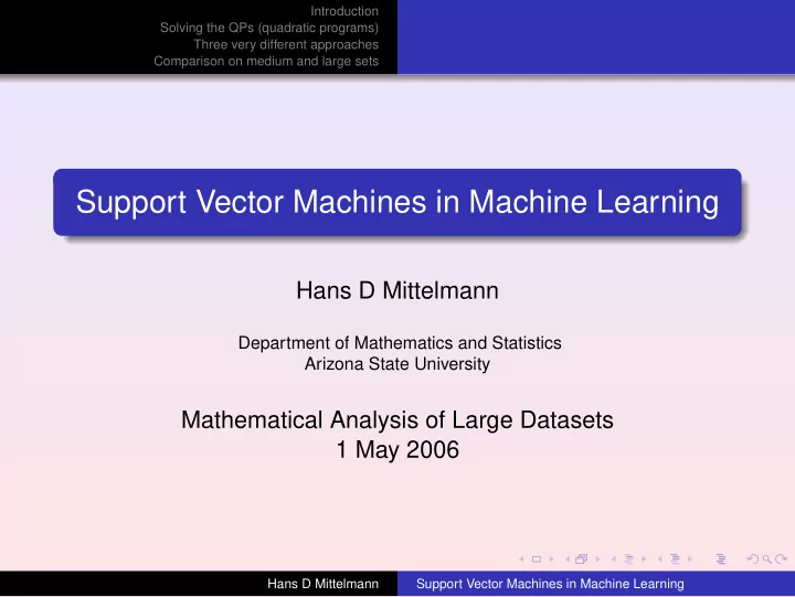
Introduction Solving the QPs (quadratic programs) Three very different approaches Comparison on medium and large sets Support Vector Machines in Machine Learning Hans D Mittelmann Department of Mathematics and Statistics Arizona State University Mathematical Analysis of Large Datasets 1 May 2006 Hans D Mittelmann Support Vector Machines in Machine Learning
Introduction Solving the QPs (quadratic programs) Three very different approaches Comparison on medium and large sets Outline Introduction 1 What is Machine Learning? Solving the QPs (quadratic programs) 2 The Computational Part Three very different approaches 3 Rather concise explanations Comparison on medium and large sets 4 REAL data! All with RBF kernel Hans D Mittelmann Support Vector Machines in Machine Learning
Introduction Solving the QPs (quadratic programs) What is Machine Learning? Three very different approaches Comparison on medium and large sets Outline Introduction 1 What is Machine Learning? Solving the QPs (quadratic programs) 2 The Computational Part Three very different approaches 3 Rather concise explanations Comparison on medium and large sets 4 REAL data! All with RBF kernel Hans D Mittelmann Support Vector Machines in Machine Learning
Introduction Solving the QPs (quadratic programs) What is Machine Learning? Three very different approaches Comparison on medium and large sets Which tasks in Machine Learning? How are Support Vector Machines used? We consider classification and testing of data in areas such as: computer processing of handwriting (USPS etc) speech recognition identification of faces, irises etc spam filtering categorization of newspaper articles analysis of medical or experimental data We borrowed the following introductory slides: Hans D Mittelmann Support Vector Machines in Machine Learning
History of SVM � SVM is a classifier derived from statistical learning theory by Vapnik and Chervonenkis � SVM was first introduced in COLT-92 � SVM becomes famous when, using pixel maps as input, it gives accuracy comparable to sophisticated neural networks with elaborated features in a handwriting recognition task � Currently, SVM is closely related to: � Kernel methods, large margin classifiers, reproducing kernel Hilbert space, Gaussian process 03/03/06 CSE 802. Prepared by Martin Law 4
Two Class Problem: Linear Separable Case � Many decision boundaries can Class 2 separate these two classes � Which one should we choose? Class 1 03/03/06 CSE 802. Prepared by Martin Law 5
Example of Bad Decision Boundaries Class 2 Class 2 Class 1 Class 1 03/03/06 CSE 802. Prepared by Martin Law 6
Good Decision Boundary: Margin Should Be Large � The decision boundary should be as far away from the data of both classes as possible � We should maximize the margin, m Class 2 m Class 1 03/03/06 CSE 802. Prepared by Martin Law 7
The Optimization Problem � Let { x 1 , ..., x n } be our data set and let y i ∈ { 1,-1} be the class label of x i � The decision boundary should classify all points correctly ⇒ � A constrained optimization problem 03/03/06 CSE 802. Prepared by Martin Law 8
The Optimization Problem � We can transform the problem to its dual � This is a quadratic programming (QP) problem � Global maximum of α i can always be found � w can be recovered by 03/03/06 CSE 802. Prepared by Martin Law 9
Characteristics of the Solution � Many of the α i are zero � w is a linear combination of a small number of data � Sparse representation � x i with non-zero α i are called support vectors (SV) � The decision boundary is determined only by the SV � Let t j ( j = 1, ..., s ) be the indices of the s support vectors. We can write � For testing with a new data z � Compute and classify z as class 1 if the sum is positive, and class 2 otherwise 03/03/06 CSE 802. Prepared by Martin Law 10
A Geometrical Interpretation Class 2 α 10 = 0 α 8 = 0.6 α 7 = 0 α 2 = 0 α 5 = 0 α 1 = 0.8 α 4 = 0 α 6 = 1.4 α 9 = 0 α 3 = 0 Class 1 03/03/06 CSE 802. Prepared by Martin Law 11
Some Notes � There are theoretical upper bounds on the error on unseen data for SVM � The larger the margin, the smaller the bound � The smaller the number of SV, the smaller the bound � Note that in both training and testing, the data are referenced only as inner product, x T y � This is important for generalizing to the non-linear case 03/03/06 CSE 802. Prepared by Martin Law 12
How About Not Linearly Separable � We allow “error” ξ i in classification Class 2 Class 1 03/03/06 CSE 802. Prepared by Martin Law 13
Soft Margin Hyperplane � Define ξ i = 0 if there is no error for x i � ξ i are just “slack variables” in optimization theory � We want to minimize � C : tradeoff parameter between error and margin � The optimization problem becomes 03/03/06 CSE 802. Prepared by Martin Law 14
The Optimization Problem � The dual of the problem is � w is also recovered as � The only difference with the linear separable case is that there is an upper bound C on α i � Once again, a QP solver can be used to find α i 03/03/06 CSE 802. Prepared by Martin Law 15
Extension to Non-linear Decision Boundary � Key idea: transform x i to a higher dimensional space to “make life easier” � Input space: the space x i are in � Feature space: the space of φ ( x i ) after transformation � Why transform? � Linear operation in the feature space is equivalent to non-linear operation in input space � The classification task can be “easier” with a proper transformation. Example: XOR 03/03/06 CSE 802. Prepared by Martin Law 16
Extension to Non-linear Decision Boundary � Possible problem of the transformation � High computation burden and hard to get a good estimate � SVM solves these two issues simultaneously � Kernel tricks for efficient computation � Minimize || w || 2 can lead to a “good” classifier φ ( ) φ ( ) φ ( ) φ ( ) φ ( ) φ (.) φ ( ) φ ( ) φ ( ) φ ( ) φ ( ) φ ( ) φ ( ) φ ( ) φ ( ) φ ( ) φ ( ) φ ( ) φ ( ) Feature space Input space 03/03/06 CSE 802. Prepared by Martin Law 17
Example Transformation � Define the kernel function K ( x , y ) as � Consider the following transformation � The inner product can be computed by K without going through the map φ (.) 03/03/06 CSE 802. Prepared by Martin Law 18
Kernel Trick � The relationship between the kernel function K and the mapping φ (.) is � This is known as the kernel trick � In practice, we specify K , thereby specifying φ (.) indirectly, instead of choosing φ (.) � Intuitively, K ( x , y ) represents our desired notion of similarity between data x and y and this is from our prior knowledge � K ( x , y ) needs to satisfy a technical condition (Mercer condition) in order for φ (.) to exist 03/03/06 CSE 802. Prepared by Martin Law 19
Examples of Kernel Functions � Polynomial kernel with degree d � Radial basis function kernel with width σ � Closely related to radial basis function neural networks � Sigmoid with parameter κ and θ � It does not satisfy the Mercer condition on all κ and θ � Research on different kernel functions in different applications is very active 03/03/06 CSE 802. Prepared by Martin Law 20
Example of SVM Applications: Handwriting Recognition 03/03/06 CSE 802. Prepared by Martin Law 21
Modification Due to Kernel Function � Change all inner products to kernel functions � For training, Original With kernel function 03/03/06 CSE 802. Prepared by Martin Law 22
Modification Due to Kernel Function � For testing, the new data z is classified as class 1 if f ≥ 0, and as class 2 if f < 0 Original With kernel function 03/03/06 CSE 802. Prepared by Martin Law 23
Example � Suppose we have 5 1D data points � x 1 = 1, x 2 = 2, x 3 = 4, x 4 = 5, x 5 = 6, with 1, 2, 6 as class 1 and 4, 5 as class 2 ⇒ y 1 = 1, y 2 = 1, y 3 = -1, y 4 = -1, y 5 = 1 � We use the polynomial kernel of degree 2 � K(x,y) = (xy+ 1) 2 � C is set to 100 � We first find α i ( i = 1, …, 5) by 03/03/06 CSE 802. Prepared by Martin Law 24
Example � By using a QP solver, we get � α 1 = 0, α 2 = 2.5, α 3 = 0, α 4 = 7.333, α 5 = 4.833 � Note that the constraints are indeed satisfied � The support vectors are { x 2 = 2, x 4 = 5, x 5 = 6} � The discriminant function is � b is recovered by solving f(2)= 1 or by f(5)= -1 or by f(6)= 1 , as x 2 , x 4 , x 5 lie on and all give b= 9 03/03/06 CSE 802. Prepared by Martin Law 25
Example Value of discriminant function class 1 class 1 class 2 1 2 4 5 6 03/03/06 CSE 802. Prepared by Martin Law 26
Multi-class Classification � SVM is basically a two-class classifier � One can change the QP formulation to allow multi-class classification � More commonly, the data set is divided into two parts “intelligently” in different ways and a separate SVM is trained for each way of division � Multi-class classification is done by combining the output of all the SVM classifiers � Majority rule � Error correcting code � Directed acyclic graph 03/03/06 CSE 802. Prepared by Martin Law 27
Recommend
More recommend
Explore More Topics
Stay informed with curated content and fresh updates.
