State space models Convenient description of dynamical systems that - PowerPoint PPT Presentation

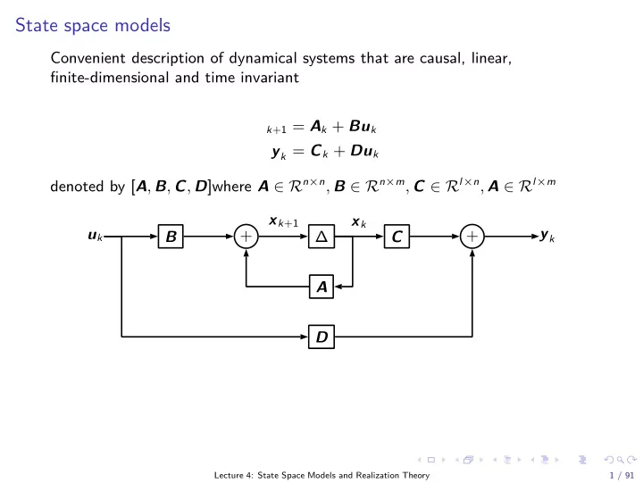
State space models Convenient description of dynamical systems that are causal, linear, finite-dimensional and time invariant k + 1 = A k + Bu k y k = C k + Du k denoted by [ A , B , C , D ] where A ∈ R n × n , B ∈ R n × m , C ∈ R l × n , A ∈ R l × m x k + 1 x k y k u k + + ∆ B C A D Lecture 4: State Space Models and Realization Theory 1 / 91

Transfer function Apply the z -transformation z X ( z ) − z x 0 = AX ( z ) + BU ( z ) Y ( z ) = CX ( z ) + DU ( z ) Investigating input-output relations, we need to eliminate X ( z ) Y ( z ) = � C ( z I − A ) − 1 B + D � + C ( z I − A ) − 1 z x 0 Assume x 0 = 0, then Y ( z ) = G ( z ) U ( z ) G ( z ) = C ( z I − A ) − 1 B + D we call G ( z ) the transfer function matrix Lecture 4: State Space Models and Realization Theory 2 / 91

Inverse transfer function Assume D invertible (only if number of inputs and outputs are the same!) G = [ A , B , C , D ] � G − 1 = [ A − BD − 1 C , BD − 1 , − D − 1 C , D − 1 ] G : Transformed outputs can be obtained as a linear transformation of the inputs G − 1 : Inputs can be obtained as a linear transformation of the transformed outputs Lecture 4: State Space Models and Realization Theory 3 / 91

Similarity transform Transfer function is unique, but state space model is not! x k = Tw k where w k ∈ R n , T ∈ R n × n w k + 1 = ( T − 1 AT ) w k + T − 1 Bu k y k = ( CT ) w k + Du k Same transfer function, but [ A , B , C , D ] � = [ T − 1 AT , T − 1 B , CT , D ] Note than under similarity transforms Λ( A ) = Λ( T − 1 AT ) Lecture 4: State Space Models and Realization Theory 4 / 91

Poles The eigenvalues λ i , i = 1 , . . . , n of the system matrix A are called the poles of a state space description [ A , B , C , D ] of the system. The pole polynomial is defined as n � π ( z ) = ( z − λ i ) i = 1 Poles of a transfer natrix G ( z ) of a system are the values of z where at least one of the entries of G ( z ) is infinite Since G ( z ) = C ( z I − A ) − 1 B + D poles of transfer matrix = poles of the state space description! Lecture 4: State Space Models and Realization Theory 5 / 91

Poles Why are poles interesting? 1. They are system invariants, like the transfer function matrix 2. Stability 3. Observability 4. Controllability Lecture 4: State Space Models and Realization Theory 6 / 91

Zeros Normal rank of G ( z ) is the ‘generic’ rank of G ( z ) , i.e. the rank of G ( z ) for almost all complex numbers z ∈ C , except for a finite number, called zeros of the transfer matrix Zeros z ∈ C lower the rank of G ( z ) rank ( G ( z )) < normal rank Zeros can be computed as the eigenvalues of A − BD − 1 C , therefore finite in number Note that when D is invertible, the zeros of G are the poles of G − 1 Lecture 4: State Space Models and Realization Theory 7 / 91

Zero structure at infinity Mapping of complex plane onto itself and move point at s = ∞ to the point λ = − δ/γ using s = ( αλ + β )( γλ + δ ) − 1 � � αλ + β ¯ G ( λ ) = G γλ + δ Zero structure at infinity can be deduced from zero structure at λ 0 = δ/γ, γ � = 0 and λ 0 does not coincide with a pole of G ( z ) The zero polynomial is defined as � ξ ( z ) = ( z − ξ i ) i where the product is over all zeros Lecture 4: State Space Models and Realization Theory 8 / 91

Zeros Poles and zeros can coincide in a multivariable system without cancelling in the transfer matrix Example � z − 1 � 0 G ( z ) = z z + 1 0 z − 1 with zeros 1 and -1, poles 0 and 1 Example � � 1 1 G ( z ) = z 0 1 with a pole and zero at 0 When G ( z ) ∈ R l × l with rank l, poles of G are zeros of G − 1 Lecture 4: State Space Models and Realization Theory 9 / 91

Computing zeros Zeros of a MIMO 1 via generalized eigenvalue decomposition If ξ causes G ( ξ ) to drop rank, and ξ not a pole, then ( D + C ( ξ I − A ) − 1 B ) v = 0 Denote u = ( ξ I − A ) − 1 Bv , then � � � � � � � � A B u I 0 u = ξ C D v 0 0 v If D is invertible, v = − D − 1 Cu ( A − BD − 1 C ) u = u ξ 1 multiple input, multiple output Lecture 4: State Space Models and Realization Theory 10 / 91

Computing zeros System with two inputs, two outputs � 1 . 9 � � � − 1 . 68 0 . 49 1 2 C = � � D = � 1 � 2 1 . 5 − 5 0 1 0 0 0 . 5 3 A = B = − 1 − 2 3 0 0 0 1 0 − 1 2 with transfer matrix � � ( z + 7 . 6609 )( z 2 − 1 . 8109 z + 0 . 9679 ) ( z + 7 . 02664 )( z − 0 . 5797 ) ( z 2 − 1 . 6860 z + 0 . 8310 ) ( z − 3 . 9695 )( z − 0 . 5605 ) G ( z ) = ( z − 0 . 5 )( z 2 − 1 . 4 z + 0 . 98 ) D is not invertible, the generalized eigenvalue problen >> eig ([A B; C D],diag([1 1 1 0 0]) ) gives us -7.9471, 0.9771, ∞ Lecture 4: State Space Models and Realization Theory 11 / 91

Physical interpretation of poles and zeros What about the generalized eigenvectors? For a zero ξ we find vectors x 0 and u 0 such that � � � � ξ I − A − B x 0 = 0 C D u 0 from which we can construct an input u k = u 0 ξ k k ≤ 0 In combination with the initial state vector x 0 the response is y k = 0 k ≤ 0 Lecture 4: State Space Models and Realization Theory 12 / 91

Physical interpretation of poles and zeros y 0 = Cx 0 + Du 0 = 0 x 1 = Ax 0 + Bu 0 = ξ x 0 y 1 = Cx 1 + Du 1 = ξ ( Cx 0 + Du 0 ) = 0 x 2 = Ax 1 + Bu 1 = ξ ( Ax 0 + Bu 0 ) = ξ 2 x 0 . . . Lecture 4: State Space Models and Realization Theory 13 / 91

Physical interpretation of poles and zeros A = � 1 . 3 � B = � 1 � C = � 1 � D = � 0 � − 0 . 4 1 0 . 6 0 1 0 0 0 2 1 0 1 Generalized eigenvalue problem finds zero at ξ = − 0 . 6 >> sys = ss ([1.3 -0.4; 1 0],[1 1; 0 0],[1 0.6; 2 -1],[0 0; 0 1],1) ; >> u = u0*(xi.^t); >> [y,t,x] = lsim(sys ,u,t,x0); In(1) State(1) Out(1) 1 1 1 0.5 0.5 0.5 0 0 0 −0.5 −0.5 −0.5 −1 −1 −1 0 5 10 15 20 0 5 10 15 20 0 5 10 15 20 In(2) State(2) Out(2) 1 1 1 0.5 0.5 0.5 0 0 0 −0.5 −0.5 −0.5 −1 −1 −1 0 5 10 15 20 0 5 10 15 20 0 5 10 15 20 Lecture 4: State Space Models and Realization Theory 14 / 91

Physical interpretation of poles and zeros If l ≥ m , there are m − l + 1 linear independent vectors u 0 , u 1 , . . . , u m − l orthogonal to G ( ξ ) G ( ξ ) � � u 0 u 1 . . . u m − l = matx 0 The set of all rational m × 1 vectors f ( z ) such that G ( z ) f ( z ) = 0 is called the right null-space of G ( z ) Every element of the right null-space is orthogonal to the row of G ( z ) and the dimension is m − r , r is the normal rank of G ( z ) Lecture 4: State Space Models and Realization Theory 15 / 91

Physical interpretation of poles and zeros Example: poles and zeros in the z -domain for transfer function z 2 + 1 . 8 z + 0 . 85 G ( z ) = z 3 − 0 . 9 z 2 + 0 . 51 z + 0 . 061 with zeros at: − 0 . 9 ± 0 . 2 i and poles at: 0 . 5 ± 0 . 6 i and − 0 . 1 40 20 dB 0 −20 −40 1 0.5 1 0.5 0 0 −0.5 −0.5 −1 −1 x y Lecture 4: State Space Models and Realization Theory 16 / 91

Impulse response of a system Assume initial state x 0 = 0 for state space equations k + 1 = A k + Bu k y k = C k + Du k Impulse input sequence at i -th component gives output y 0 = d i y 1 = Cb i y 2 = CAb i . . . y k = CA k − 1 b i Lecture 4: State Space Models and Realization Theory 17 / 91

Impulse response of a system Impulse response matrices/Markov parameters H 0 = D H 1 = CB H 2 = CAB . . . H k = CA k − 1 B Similarity transformation x k = Tw k H k = CA k − 1 B = ( CT )( T − 1 A k − 1 T )( T − 1 B ) k = 1 , 2 , . . . Impulse response matrices are invariants of a system! Lecture 4: State Space Models and Realization Theory 18 / 91

Impulse response of a system Example: >> A = [2 -1.83 0.794 -0.185; 1 0 0 0; 0 1 0 0; 0 0 1 0]; >> B = [1 0 -1; 2 -1 3; 0 -0.5 1; 3 -2 0]; >> C = [1 0 0 2; -5 1 -4 0; 0 7 6 -3; 3 -2 4 5]; >> D = [0 1 0; 1 0 0; 0 0 -1; 1 2 0]; >> sys = ss(A,B,C,D,1) ; >> impulse(sys) Impulse Response From: In(1) From: In(2) From: In(3) 20 To: Out(1) 0 −20 100 To: Out(2) 0 Amplitude −100 200 To: Out(3) 0 −200 100 To: Out(4) 0 −100 0 20 40 0 20 40 0 20 40 Time (seconds) Lecture 4: State Space Models and Realization Theory 19 / 91

Modal decomposition Let A have an eigenvalue decomposition XJX − 1 Similarity transform with T = X gives [ A , B , C , D ] → [ J , X − 1 B , CX , D ] Matrix J reveals the system poles and their multiplicity Lecture 4: State Space Models and Realization Theory 20 / 91

Modal decomposition Case 1: A is diagonalizable; left and right eigenvectors of A Ap i = p i λ i A t q i = q i λ i normalized such that q t i p i = 1. It can be shown that n � R i z X ( z ) = ( z I − A ) − 1 z x 0 = z − λ i x 0 i = 1 with R i = p i q ∗ i . By rearranging and taking the z -transform n � α i λ k x k = i p i i = 1 where α i = q t i x 0 . This is the modal decomposition . Lecture 4: State Space Models and Realization Theory 21 / 91