Introduction to State Space Methods Siem Jan Koopman - PowerPoint PPT Presentation
Introduction to State Space Methods Siem Jan Koopman s.j.koopman@feweb.vu.nl Vrije Universiteit Amsterdam Tinbergen Institute Introduction to State Space Methods p. 1 State Space Model Linear Gaussian state space model is defined in three
Introduction to State Space Methods Siem Jan Koopman s.j.koopman@feweb.vu.nl Vrije Universiteit Amsterdam Tinbergen Institute Introduction to State Space Methods – p. 1
State Space Model Linear Gaussian state space model is defined in three parts: → State equation: ζ t ∼ NID (0 , Q t ) , α t +1 = T t α t + R t ζ t , → Observation equation: y t = Z t α t + ε t , ε t ∼ NID (0 , G t ) , → Initial state distribution α 1 ∼ N ( a 1 , P 1 ) . Notice that • ζ t and ε s independent for all t, s , and independent from α 1 ; • observation y t can be multivariate; • state vector α t is unobserved; • matrices T t , Z t , R t , Q t , G t determine structure of model. Introduction to State Space Methods – p. 2
State Space Model • state space model is linear and Gaussian: therefore properties and results of multivariate normal distribution apply; • state vector α t evolves as a VAR(1) process; • system matrices usually contain unknown parameters; • estimation has therefore two aspects: ◦ measuring the unobservable state (prediction, filtering and smoothing); ◦ estimation of unknown parameters (maximum likelihood estimation); • state space methods offer a unified approach to a wide range of models and techniques: dynamic regression, ARIMA, UC models, latent variable models, spline-fitting and many ad-hoc filters; • next, some well-known model specifications in state space form ... Introduction to State Space Methods – p. 3
Regression with Time Varying Coefficients General state space model: ζ t ∼ NID (0 , Q t ) , α t +1 = T t α t + R t ζ t , y t = Z t α t + ε t , ε t ∼ NID (0 , G t ) . Put regressors in Z t , T t = I, R t = I, Result is regression model with coefficient α t following a random walk. Introduction to State Space Methods – p. 4
ARMA in State Space Form Example: AR(2) model y t +1 = φ 1 y t + φ 2 y t − 1 + ζ t , in state space: α t +1 = T t α t + R t ζ t , ζ t ∼ NID (0 , Q t ) , ε t ∼ NID (0 , G t ) . y t = Z t α t + ε t , with 2 × 1 state vector α t and system matrices: � � Z t = , G t = 0 1 0 � � � � φ 1 1 1 Q t = σ 2 T t = , R t = , φ 2 0 0 • Z t and G t = 0 imply that α 1 t = y t ; • First state equation implies y t +1 = φ 1 y t + α 2 t + ζ t with ζ t ∼ NID (0 , σ 2 ) ; • Second state equation implies α 2 ,t +1 = φ 2 y t ; Introduction to State Space Methods – p. 5
ARMA in State Space Form Example: MA(1) model y t +1 = ζ t + θζ t − 1 , in state space: α t +1 = T t α t + R t ζ t , ζ t ∼ NID (0 , Q t ) , ε t ∼ NID (0 , G t ) . y t = Z t α t + ε t , with 2 × 1 state vector α t and system matrices: � � Z t = , G t = 0 1 0 � � � � 0 1 1 Q t = σ 2 T t = , R t = , 0 0 θ • Z t and G t = 0 imply that α 1 t = y t ; • First state equation implies y t +1 = α 2 t + ζ t with ζ t ∼ NID (0 , σ 2 ) ; • Second state equation implies α 2 ,t +1 = θζ t ; Introduction to State Space Methods – p. 6
ARMA in State Space Form Example: ARMA(2,1) model y t = φ 1 y t − 1 + φ 2 y t − 2 + ζ t + θζ t − 1 in state space form � � y t α t = φ 2 y t − 1 + θζ t � � Z t = , G t = 0 , 1 0 � � � � φ 1 1 1 Q t = σ 2 T t = , R t = , φ 2 0 θ All ARIMA ( p, d, q ) models have a (non-unique) state space representation. Introduction to State Space Methods – p. 7
UC models in State Space Form State space model: α t +1 = T t α t + R t ζ t , y t = Z t α t + ε t . LL model ∆ µ t +1 = η t and y t = µ t + ε t : Q t = σ 2 α t = µ t , T t = 1 , R t = 1 , η , G t = σ 2 Z t = 1 , ε . LLT model ∆ µ t +1 = β t + η t , ∆ β t +1 = ξ t and y t = µ t + ε t : � � � � � � � � σ 2 µ t 1 1 1 0 0 η α t = , T t = , R t = , Q t = , σ 2 β t 0 1 0 1 0 ξ � � G t = σ 2 Z t = , ε . 1 0 Introduction to State Space Methods – p. 8
UC models in State Space Form State space model: α t +1 = T t α t + R t ζ t , y t = Z t α t + ε t . LLT model with season: ∆ µ t +1 = β t + η t , ∆ β t +1 = ξ t , S ( L ) γ t +1 = ω t and y t = µ t + γ t + ε t : � ′ � α t = , µ t β t γ t γ t − 1 γ t − 2 1 1 0 0 0 1 0 0 σ 2 0 1 0 0 0 0 0 0 1 0 η σ 2 T t = − 1 − 1 − 1 , Q t = , R t = , 0 0 0 0 0 0 1 ξ σ 2 0 0 1 0 0 0 0 0 0 0 ω 0 0 0 1 0 0 0 0 � � G t = σ 2 Z t = , ε . 1 0 1 0 0 Introduction to State Space Methods – p. 9
Kalman Filter • The Kalman filter calculates the mean and variance of the unobserved state, given the observations. • The state is Gaussian: the complete distribution is characterized by the mean and variance. • The filter is a recursive algorithm; the current best estimate is updated whenever a new observation is obtained. • To start the recursion, we need a 1 and P 1 , which we assumed given. • There are various ways to initialize when a 1 and P 1 are unknown, which we will not discuss here. Introduction to State Space Methods – p. 10
Kalman Filter The unobserved state α t can be estimated from the observations with the Kalman filter : v t = y t − Z t a t , F t = Z t P t Z ′ t + G t , t F − 1 K t = T t P t Z ′ , t a t +1 = T t a t + K t v t , P t +1 = T t P t T ′ t + R t Q t R ′ t − K t F t K ′ t , for t = 1 , . . . , n and starting with given values for a 1 and P 1 . • Writing Y t = { y 1 , . . . , y t } , a t +1 = E( α t +1 | Y t ) , P t +1 = var( α t +1 | Y t ) . Introduction to State Space Methods – p. 11
Kalman Filter State space model: α t +1 = T t α t + R t ζ t , y t = Z t α t + ε t . • Writing Y t = { y 1 , . . . , y t } , define a t +1 = E( α t +1 | Y t ) , P t +1 = var( α t +1 | Y t ); • The prediction error is v t = y t − E( y t | Y t − 1 ) = y t − E( Z t α t + ε t | Y t − 1 ) = y t − Z t E( α t | Y t − 1 ) = y t − Z t a t ; • It follows that v t = Z t ( α t − a t ) + ε t and E( v t ) = 0 ; • The prediction error variance is F t = var( v t ) = Z t P t Z ′ t + G t . Introduction to State Space Methods – p. 12
Lemma The proof of the Kalman filter uses a lemma from multivariate Normal regression theory. Lemma Suppose x, y and z are jointly Normally distributed vectors with E( z ) = 0 and Σ yz = 0 . Then E( x | y, z ) = E( x | y ) + Σ xz Σ − 1 zz z, var( x | y, z ) = var( x | y ) − Σ xz Σ − 1 zz Σ ′ xz , Introduction to State Space Methods – p. 13
Kalman Filter State space model: α t +1 = T t α t + R t ζ t , y t = Z t α t + ε t . • We have Y t = { Y t − 1 , y t } = { Y t − 1 , v t } and E( v t y t − j ) = 0 for j = 1 , . . . , t − 1 ; • Lemma E( x | y, z ) = E( x | y ) + Σ xz Σ − 1 zz z , and take x = α t +1 , y = Y t − 1 and z = v t = Z t ( α t − a t ) + ε t ; • It follows that E( α t +1 | Y t − 1 ) = T t a t ; • Furter, E( α t +1 v ′ t ) = T t E( α t v ′ t ) + R t E( ζ t v ′ t ) = T t P t Z ′ t ; • We carry out lemma and obtain the state update a t +1 = E( α t +1 | Y t − 1 , y t ) t F − 1 = T t a t + T t P t Z ′ v t t = T t a t + K t v t ; t F − 1 with K t = T t P t Z ′ t Introduction to State Space Methods – p. 14
Kalman Filter Our best prediction of y t is Z t a t . When the actual observation arrives, calculate the prediction error v t = y t − Z t a t and its variance F t = Z t P t Z ′ t + G t . The new best estimates of the state mean is based on both the old estimate a t and the new information v t : a t +1 = T t a t + K t v t , similarly for the variance: P t +1 = T t P t T ′ t + R t Q t R ′ t − K t F t K ′ t . The Kalman gain t F − 1 K t = T t P t Z ′ t is the optimal weighting matrix for the new evidence. Introduction to State Space Methods – p. 15
Kalman Filter Illustration 10000 observation filtered level a_t state variance P_t 1250 9000 1000 8000 7000 750 6000 500 1880 1900 1920 1940 1960 1880 1900 1920 1940 1960 prediction error v_t prediction error variance F_t 25000 250 24000 0 23000 22000 −250 21000 1880 1900 1920 1940 1960 1880 1900 1920 1940 1960 Introduction to State Space Methods – p. 16
Smoothing • The filter calculates the mean and variance conditional on Y t ; • The Kalman smoother calculates the mean and variance conditional on the full set of observations Y n ; • After the filtered estimates are calculated, the smoothing recursion starts at the last observations and runs until the first. α t = E( α t | Y n ) , ˆ V t = var( α t | Y t ) , r t = weighted sum of innovations , N t = var( r t ) , L t = T t − K t Z t . Starting with r n = 0 , N n = 0 , the smoothing recursions are given by r t − 1 = F − 1 N t − 1 = F − 1 + L 2 v t + L t r t , t N t , t t V t = P t − P 2 α t = a t + P t r t − 1 , ˆ t N t − 1 . Introduction to State Space Methods – p. 17
Smoothing Illustration 4000 observations smoothed state V_t 1250 3500 1000 3000 750 2500 500 1880 1900 1920 1940 1960 1880 1900 1920 1940 1960 0.000100 0.02 r_t N_t 0.000075 0.00 0.000050 −0.02 0.000025 1880 1900 1920 1940 1960 1880 1900 1920 1940 1960 Introduction to State Space Methods – p. 18
Recommend
More recommend
Explore More Topics
Stay informed with curated content and fresh updates.
