Stat 5421 Lecture Notes: To Accompany Agresti Ch 4, Addendum Charles - PDF document
Stat 5421 Lecture Notes: To Accompany Agresti Ch 4, Addendum Charles J. Geyer October 21, 2020 Intercept Makes No Difference When Any Predictor Is Categorical We use for an example data from the examples for R function glm ## Dobson (1990) Page
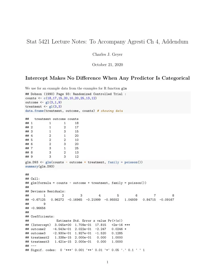
Stat 5421 Lecture Notes: To Accompany Agresti Ch 4, Addendum Charles J. Geyer October 21, 2020 Intercept Makes No Difference When Any Predictor Is Categorical We use for an example data from the examples for R function glm ## Dobson (1990) Page 93: Randomized Controlled Trial : counts <- c (18,17,15,20,10,20,25,13,12) outcome <- gl (3,1,9) treatment <- gl (3,3) data.frame (treatment, outcome, counts) # showing data ## treatment outcome counts ## 1 1 1 18 ## 2 1 2 17 ## 3 1 3 15 ## 4 2 1 20 ## 5 2 2 10 ## 6 2 3 20 ## 7 3 1 25 ## 8 3 2 13 ## 9 3 3 12 glm.D93 <- glm (counts ~ outcome + treatment, family = poisson ()) summary (glm.D93) ## ## Call: ## glm(formula = counts ~ outcome + treatment, family = poisson()) ## ## Deviance Residuals: ## 1 2 3 4 5 6 7 8 ## -0.67125 0.96272 -0.16965 -0.21999 -0.95552 1.04939 0.84715 -0.09167 ## 9 ## -0.96656 ## ## Coefficients: ## Estimate Std. Error z value Pr(>|z|) ## (Intercept) 3.045e+00 1.709e-01 17.815 <2e-16 *** ## outcome2 -4.543e-01 2.022e-01 -2.247 0.0246 * ## outcome3 -2.930e-01 1.927e-01 -1.520 0.1285 ## treatment2 1.338e-15 2.000e-01 0.000 1.0000 ## treatment3 1.421e-15 2.000e-01 0.000 1.0000 ## --- ## Signif. codes: 0 '***' 0.001 '**' 0.01 '*' 0.05 '.' 0.1 ' ' 1 1
## ## (Dispersion parameter for poisson family taken to be 1) ## ## Null deviance: 10.5814 on 8 degrees of freedom ## Residual deviance: 5.1291 on 4 degrees of freedom ## AIC: 56.761 ## ## Number of Fisher Scoring iterations: 4 Note that outcome and treatment are factors (the terminology R uses for categorical variables) class (outcome) ## [1] "factor" class (treatment) ## [1] "factor" and they each have three levels nlevels (outcome) ## [1] 3 nlevels (treatment) ## [1] 3 So how does a categorical variable correspond to a regression model in which it is used. For each categorical variable, the regression model needs dummy variables , one for each category (R calls them levels of the factor variable). We can see these dummy variables as follows model.matrix ( ~ 0 + outcome) ## outcome1 outcome2 outcome3 ## 1 1 0 0 ## 2 0 1 0 ## 3 0 0 1 ## 4 1 0 0 ## 5 0 1 0 ## 6 0 0 1 ## 7 1 0 0 ## 8 0 1 0 ## 9 0 0 1 ## attr(,"assign") ## [1] 1 1 1 ## attr(,"contrasts") ## attr(,"contrasts")$outcome ## [1] "contr.treatment" model.matrix ( ~ 0 + treatment) ## treatment1 treatment2 treatment3 ## 1 1 0 0 ## 2 1 0 0 ## 3 1 0 0 ## 4 0 1 0 ## 5 0 1 0 ## 6 0 1 0 2
## 7 0 0 1 ## 8 0 0 1 ## 9 0 0 1 ## attr(,"assign") ## [1] 1 1 1 ## attr(,"contrasts") ## attr(,"contrasts")$treatment ## [1] "contr.treatment" Each dummy variable indicates the cases (components of the response vector, rows of the model matrix) which are in that category (level). Note that the dummy variables corresponding to a categorical variable add up to the vector all of whose components are equal to one, which is what R calls the intercept dummy variable. rowSums ( model.matrix ( ~ 0 + outcome)) ## 1 2 3 4 5 6 7 8 9 ## 1 1 1 1 1 1 1 1 1 rowSums ( model.matrix ( ~ 0 + treatment)) ## 1 2 3 4 5 6 7 8 9 ## 1 1 1 1 1 1 1 1 1 model.matrix (counts ~ 1) ## (Intercept) ## 1 1 ## 2 1 ## 3 1 ## 4 1 ## 5 1 ## 6 1 ## 7 1 ## 8 1 ## 9 1 ## attr(,"assign") ## [1] 0 Thus we would not have an identifiable model if we kept all of the dummy variables corresponding to a categorical variable and kept an “intercept” dummy variable. The default behavior in R is to • keep an “intercept” dummy variable and • drop one of the dummy variables for each categorical variable (factor). This gives an identifiable model. model.matrix (counts ~ outcome + treatment) ## (Intercept) outcome2 outcome3 treatment2 treatment3 ## 1 1 0 0 0 0 ## 2 1 1 0 0 0 ## 3 1 0 1 0 0 ## 4 1 0 0 1 0 ## 5 1 1 0 1 0 ## 6 1 0 1 1 0 ## 7 1 0 0 0 1 ## 8 1 1 0 0 1 3
## 9 1 0 1 0 1 ## attr(,"assign") ## [1] 0 1 1 2 2 ## attr(,"contrasts") ## attr(,"contrasts")$outcome ## [1] "contr.treatment" ## ## attr(,"contrasts")$treatment ## [1] "contr.treatment" The dummy variables outcome1 and treatment1 are omitted. But we can tell R to omit the intercept. model.matrix (counts ~ 0 + outcome + treatment) ## outcome1 outcome2 outcome3 treatment2 treatment3 ## 1 1 0 0 0 0 ## 2 0 1 0 0 0 ## 3 0 0 1 0 0 ## 4 1 0 0 1 0 ## 5 0 1 0 1 0 ## 6 0 0 1 1 0 ## 7 1 0 0 0 1 ## 8 0 1 0 0 1 ## 9 0 0 1 0 1 ## attr(,"assign") ## [1] 1 1 1 2 2 ## attr(,"contrasts") ## attr(,"contrasts")$outcome ## [1] "contr.treatment" ## ## attr(,"contrasts")$treatment ## [1] "contr.treatment" Now the behavior is • omit an “intercept” dummy variable and • drop one of the dummy variables for each categorical variable (factor) except for one categorical variable (for which we keep all of its dummy variables) Note — this is very important — that these two recipes give the same model. • Leaving out the intercept produces a different model when all of the predictor variables are quantitative . • Leaving out the intercept produces the same model when at least one of the predictor variables is categorical (qualitative, factor) . glm.D93.no.intercept <- glm (counts ~ 0 + outcome + treatment, family = poisson ()) summary (glm.D93.no.intercept) ## ## Call: ## glm(formula = counts ~ 0 + outcome + treatment, family = poisson()) ## ## Deviance Residuals: ## 1 2 3 4 5 6 7 8 4
## -0.67125 0.96272 -0.16965 -0.21999 -0.95552 1.04939 0.84715 -0.09167 ## 9 ## -0.96656 ## ## Coefficients: ## Estimate Std. Error z value Pr(>|z|) ## outcome1 3.045e+00 1.709e-01 17.82 <2e-16 *** ## outcome2 2.590e+00 1.958e-01 13.23 <2e-16 *** ## outcome3 2.752e+00 1.860e-01 14.79 <2e-16 *** ## treatment2 9.287e-19 2.000e-01 0.00 1 ## treatment3 -4.885e-16 2.000e-01 0.00 1 ## --- ## Signif. codes: 0 '***' 0.001 '**' 0.01 '*' 0.05 '.' 0.1 ' ' 1 ## ## (Dispersion parameter for poisson family taken to be 1) ## ## Null deviance: 572.6047 on 9 degrees of freedom ## Residual deviance: 5.1291 on 4 degrees of freedom ## AIC: 56.761 ## ## Number of Fisher Scoring iterations: 4 Note that the regression coefficients (estimates) are different from the ones with intercept shown above. But the estimated cell means are the same, hence the both specify the same statistical model . These are different parameterizations of the same model. mu <- predict (glm.D93, type = "response") mu.no.intercept <- predict (glm.D93.no.intercept, type = "response") all.equal (mu, mu.no.intercept) ## [1] TRUE R Function drop1 R function drop1 is useful for finding out the effect of dropping terms from a model, especially when there are categorical variables, in which case one wants to drop all of the dummy variables for a categorical variable or drop none of them. drop1 (glm.D93, test = "LRT") ## Single term deletions ## ## Model: ## counts ~ outcome + treatment ## Df Deviance AIC LRT Pr(>Chi) ## <none> 5.1291 56.761 ## outcome 2 10.5814 58.214 5.4523 0.06547 . ## treatment 2 5.1291 52.761 0.0000 1.00000 ## --- ## Signif. codes: 0 '***' 0.001 '**' 0.01 '*' 0.05 '.' 0.1 ' ' 1 5
R Function add1 There is also an R function add1 glm.D93.intercept.only <- glm (counts ~ 1, family = poisson ()) add1 (glm.D93.intercept.only, scope = ~ outcome + treatment, test = "LRT") ## Single term additions ## ## Model: ## counts ~ 1 ## Df Deviance AIC LRT Pr(>Chi) ## <none> 10.5814 54.214 ## outcome 2 5.1291 52.761 5.4523 0.06547 . ## treatment 2 10.5814 58.214 0.0000 1.00000 ## --- ## Signif. codes: 0 '***' 0.001 '**' 0.01 '*' 0.05 '.' 0.1 ' ' 1 R Function anova But one can also do these tests using R function anova glm.D93.outcome.only <- glm (counts ~ outcome, family = poisson ()) glm.D93.treatment.only <- glm (counts ~ treatment, family = poisson ()) # compare with results of drop1 anova (glm.D93.outcome.only, glm.D93, test = "LRT") ## Analysis of Deviance Table ## ## Model 1: counts ~ outcome ## Model 2: counts ~ outcome + treatment ## Resid. Df Resid. Dev Df Deviance Pr(>Chi) ## 1 6 5.1291 ## 2 4 5.1291 2 2.6645e-15 1 anova (glm.D93.treatment.only, glm.D93, test = "LRT") ## Analysis of Deviance Table ## ## Model 1: counts ~ treatment ## Model 2: counts ~ outcome + treatment ## Resid. Df Resid. Dev Df Deviance Pr(>Chi) ## 1 6 10.5814 ## 2 4 5.1291 2 5.4523 0.06547 . ## --- ## Signif. codes: 0 '***' 0.001 '**' 0.01 '*' 0.05 '.' 0.1 ' ' 1 # compare with results of add1 anova (glm.D93.intercept.only, glm.D93.outcome.only, test = "LRT") ## Analysis of Deviance Table ## ## Model 1: counts ~ 1 ## Model 2: counts ~ outcome 6
## Resid. Df Resid. Dev Df Deviance Pr(>Chi) ## 1 8 10.5814 ## 2 6 5.1291 2 5.4523 0.06547 . ## --- ## Signif. codes: 0 '***' 0.001 '**' 0.01 '*' 0.05 '.' 0.1 ' ' 1 anova (glm.D93.intercept.only, glm.D93.treatment.only, test = "LRT") ## Analysis of Deviance Table ## ## Model 1: counts ~ 1 ## Model 2: counts ~ treatment ## Resid. Df Resid. Dev Df Deviance Pr(>Chi) ## 1 8 10.581 ## 2 6 10.581 2 1.7764e-15 1 7
Recommend
More recommend
Explore More Topics
Stay informed with curated content and fresh updates.










![Git tools Sylvain Bouveret, Grgory Mouni, Matthieu Moy 2017 [first].[last]@imag.fr](https://c.sambuz.com/1075999/git-tools-s.webp)
