Intro to Categorical Data Analysis Nicholas Reich and Anna Liu, - PDF document

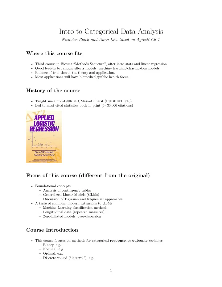
Intro to Categorical Data Analysis Nicholas Reich and Anna Liu, based on Agresti Ch 1 Where this course fits • Third course in Biostat “Methods Sequence”, after intro stats and linear regression. • Good lead-in to random effects models, machine learning/classification models. • Balance of traditional stat theory and application. • Most applications will have biomedical/public health focus. History of the course • Taught since mid-1980s at UMass-Amherst (PUBHLTH 743) • Led to most cited statistics book in print (> 30,000 citations) Focus of this course (different from the original) • Foundational concepts – Analysis of contingency tables – Generalized Linear Models (GLMs) – Discussion of Bayesian and frequentist approaches • A taste of common, modern extensions to GLMs – Machine Learning classification methods – Longitudinal data (repeated measures) – Zero-inflated models, over-dispersion Course Introduction • This course focuses on methods for categorical response , or outcome variables. – Binary, e.g. – Nominal, e.g. – Ordinal, e.g. – Discrete-valued (“interval”), e.g. 1

• Explanatory , or predictor variables can be any type • Very generally, we are trying to build models Types of categorical variables • The way that a variable is measured determines its classification – What are different ways that a variable on education could be classified? • The granularity of your data matters! – In terms of information per measured datapoint, discrete variables > ordinal variables > nominal variables – This has implications for study design and sample size. Distributions of categorical variables: Binomial Let y 1 , y 2 , · · · , y n denote observations from n independent and identical trials such that P ( Y i = 1) = π P ( Y i = 0) = 1 − π The total number of successes (1s) Y = � n i =1 Y i has the binomial distribution , denoted by bin ( n, π ). The probability mass function for the possible outcomes y for Y is � n � π y (1 − π ) ( n − y ) , y = 0 , 1 , ..., n p ( y ) = y with µ = E ( Y ) = nπ and σ 2 = V ar ( Y ) = nπ (1 − π ). • The binomial distribution converges to normality as n increases, for fixed π , the approximation being reasonable when n [min( π, 1 − π )] is as small as 5. • Interactive binomial distribution Statistical inference Inference is the use of sample data to estimate unknown parameters of the population. One method we will focus on is maximum likelihood estimation (MLE) . 2

Population Sample Population Sample Statistic Parameter Statistical inference: maximum likelihood • The likelihood function is the likelihood (or probability in the discrete case) of the sample of your data X 1 , ..., X n , given the unknown parameter(s) β . Denoted as l ( β | X 1 , ..., X n ) or simply l ( β ). • The MLE of β is defined as ˆ β = sup l ( β ) = sup L ( β ) β β where L ( β ) = log ( l ( β )). The MLE is the parameter value under which the data observed have the highest probability of occurrence. Statistical inference: MLE (con’t) • MLE have desirable properties: under weak regularity conditions, MLE have large-sample normal distributions; they are asymptotically consistent , converging to the parameter as n increases; and they are asymptotically efficient , producing large-sample standard errors no greater than those from other estimation methods. Covariance matrix of the MLE Let cov (ˆ β ) denote the asymptotic convariance matrix of ˆ β , where β is a multidimensional parameter. 3

• Under regularity conditions, cov (ˆ β ) is the inverse of the information matrix , which is � ∂ 2 L ( β ) � [ I ( β )] i,j = − E ∂β i ∂β j • The standard errors are the square roots of the diagonal elements for the inverse of the information matrix. The greater the curvature of the log likelihood function, the smaller the standard errors. Statistical inference for Binomial parameter • The binomial log likelihood function is L ( π ) = log[ π y (1 − π ) ( n − y ) ] = y log( π ) + ( n − y ) log(1 − π ) • Differentiating wrt π and setting it to 0 gives the MLE ˆ π = y/n . • The Fisher information is I ( π ) = n/ [ π (1 − π )] • The asympotic distribution of the MLE ˆ π is N ( π, π (1 − π ) /n ). Statistical inference for Binomial parameter The score, Wald, and likelihood ratio tests use different information from this curve to draw inference about π . Wald test Consider the hypothesis H 0 : β = β 0 H 1 : β � = β 0 The Wald test defines a test statistic � z = (ˆ I (ˆ � β − β 0 ) /SE, where SE = 1 / β ) = ˆ π (1 − ˆ π ) /n Under H 0 : β = β 0 , the wald test statistic z is approximately standard normal. Therefore H 0 is rejected if | z | > z α/ 2 . Likelihood ratio test The likelihood ratio test (LRT) is defined as − 2 log Λ = − 2 log( l 0 /l 1 ) = − 2( L 0 − L 1 ) where l 0 and l 1 are the maximized likelihood under H 0 and H 0 ∪ H 1 . The null hypothesis is rejected if − 2 log Λ > χ 2 α ( d f ) where d f is the difference in the dimensions of the parameter spaces under H 0 ∪ H 1 and H 0 . 4

Figure 1: binomial likelihood 5

Score (a.k.a. Wilson) test Score test , also called the Wilson or Lagrange multiplier test , is based on the slope and expected curvature of the log-likelihood function L ( β ) at the null value β 0 . It utilizes the size of the score function u ( β ) = ∂L ( β ) /∂β evaluated at β 0 . The score test statistic is u ( β 0 ) π − π 0 ˆ z = [ I ( β 0 )] 1 / 2 = � π 0 (1 − π 0 ) /n . Example: Estimating the proportion of Vegetarians Students in a class were surveyed whether they are vegetarians. Of n = 25 students, y = 0 answered “yes”. • Using the Wald method, compute the 95% confidence interval for π (true proportion of vegetarians in the population): • Using the Score method, compute the 95% confidence interval for π (true proportion of vegetarians in the population): Warning about the Wald test • When a parameter falls near the boundary of the sample space, often sample estimates of standard errors are poor and the Wald method does not provide a sensible answer. • For small to moderate sample sizes, the likelihood-ratio and score tests are usually more reliable than the Wald test, having actual error rates closer to the nominal level. Comparison of the tests There are lots of different methods to compute CIs for a binomial proportion! library (binom) binom.confint (x=0, n=25) ## method x n mean lower upper ## 1 agresti-coull 0 25 0.00000000 -0.02439494 0.15758719 ## 2 asymptotic 0 25 0.00000000 0.00000000 0.00000000 ## 3 bayes 0 25 0.01923077 0.00000000 0.07323939 ## 4 cloglog 0 25 0.00000000 0.00000000 0.13718517 ## 5 exact 0 25 0.00000000 0.00000000 0.13718517 ## 6 logit 0 25 0.00000000 0.00000000 0.13718517 ## 7 probit 0 25 0.00000000 0.00000000 0.13718517 ## 8 profile 0 25 0.00000000 0.00000000 0.12291101 ## 9 lrt 0 25 0.00000000 0.00000000 0.07398085 ## 10 prop.test 0 25 0.00000000 0.00000000 0.16577301 ## 11 wilson 0 25 0.00000000 0.00000000 0.13319225 6

Bayesian inference for binomial parameters Bayesian analyses incorporate “prior information” about parameters using • prior subjective belief about a parameter, or • prior knowledge from other studies, or • very little knowledge (a “weakly informative” prior) Prior distribution ( g ) is combined with the likelihood ( f ) to create a posterior ( h ): h ( θ | y ) = f ( y | θ ) g ( θ ) f ( y ) ∝ f ( y | θ ) g ( θ ) Using Beta distributions for priors If π ∼ beta ( α 1 , α 2 ) (for α 1 > 0 and α 2 > 0) then g ( π ) ∝ π α 1 − 1 (1 − π ) α 2 − 1 . Beta is a conjugate prior distribution for a binomial parameter, implying that the posterior is also a beta distribution, specifically, h follows a beta ( y + α 1 , n − y + α 2 ). Shiny app for Bayesian inference of a Binomial. An exercise 1. Write down your prior belief about the probability that this coin will land heads. 2. Share it with the class 3. Use the prior probabilities to estimate a beta distribution. library (MASS) x <- c ( ## enter probabilities here ) fitdistr (x, "beta", list (shape1=1,shape2=1)) 4. Use the app to see how the posterior changes as we flip the coin. 7