Stat 5421 Lecture Notes: To Accompany Agresti Ch 4 Charles J. Geyer - PDF document

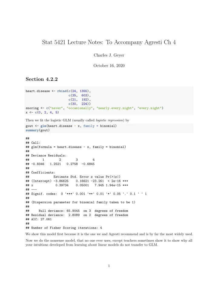
Stat 5421 Lecture Notes: To Accompany Agresti Ch 4 Charles J. Geyer October 16, 2020 Section 4.2.2 heart.disease <- rbind ( c (24, 1355), c (35, 603), c (21, 192), c (30, 224)) snoring <- c ("never", "occasionally", "nearly.every.night", "every.night") x <- c (0, 2, 4, 5) Then we fit the logistic GLM (usually called logistic regression ) by gout <- glm (heart.disease ~ x, family = binomial) summary (gout) ## ## Call: ## glm(formula = heart.disease ~ x, family = binomial) ## ## Deviance Residuals: ## 1 2 3 4 ## -0.8346 1.2521 0.2758 -0.6845 ## ## Coefficients: ## Estimate Std. Error z value Pr(>|z|) ## (Intercept) -3.86625 0.16621 -23.261 < 2e-16 *** ## x 0.39734 0.05001 7.945 1.94e-15 *** ## --- ## Signif. codes: 0 '***' 0.001 '**' 0.01 '*' 0.05 '.' 0.1 ' ' 1 ## ## (Dispersion parameter for binomial family taken to be 1) ## ## Null deviance: 65.9045 on 3 degrees of freedom ## Residual deviance: 2.8089 on 2 degrees of freedom ## AIC: 27.061 ## ## Number of Fisher Scoring iterations: 4 We show this model first because it is the one we and Agresti recommend and is by far the most widely used. Now we do the nonsense model, that no one ever uses, except teachers sometimes show it to show why all your intuitions developed from learning about linear models do not transfer to GLM. 1

gout.goofy <- glm (heart.disease ~ x, family = binomial (link="identity")) summary (gout.goofy) ## ## Call: ## glm(formula = heart.disease ~ x, family = binomial(link = "identity")) ## ## Deviance Residuals: ## 1 2 3 4 ## 0.04478 -0.21322 0.11010 0.09798 ## ## Coefficients: ## Estimate Std. Error z value Pr(>|z|) ## (Intercept) 0.017247 0.003451 4.998 5.80e-07 *** ## x 0.019778 0.002805 7.051 1.77e-12 *** ## --- ## Signif. codes: 0 '***' 0.001 '**' 0.01 '*' 0.05 '.' 0.1 ' ' 1 ## ## (Dispersion parameter for binomial family taken to be 1) ## ## Null deviance: 65.904481 on 3 degrees of freedom ## Residual deviance: 0.069191 on 2 degrees of freedom ## AIC: 24.322 ## ## Number of Fisher Scoring iterations: 3 We make a plot like Figure~4.1 in Agresti. mu <- predict (gout, type = "response") mu.goofy <- predict (gout.goofy, type = "response") mu ## 1 2 3 4 ## 0.02050742 0.04429511 0.09305411 0.13243885 mu.goofy ## 1 2 3 4 ## 0.01724668 0.05680231 0.09635793 0.11613574 plot (x, mu, ylab = "probability", pch = 19, ylim = range (mu, mu.goofy)) curve ( predict (gout, newdata = data.frame (x = x), type = "response"), add = TRUE) grep ("red", colors (), value = TRUE) ## [1] "darkred" "indianred" "indianred1" "indianred2" ## [5] "indianred3" "indianred4" "mediumvioletred" "orangered" ## [9] "orangered1" "orangered2" "orangered3" "orangered4" ## [13] "palevioletred" "palevioletred1" "palevioletred2" "palevioletred3" ## [17] "palevioletred4" "red" "red1" "red2" ## [21] "red3" "red4" "violetred" "violetred1" ## [25] "violetred2" "violetred3" "violetred4" points (x, mu.goofy, col = "red", pch = 19) curve ( predict (gout.goofy, newdata = data.frame (x = x), type = "response"), add = TRUE, col = "red") 2

0.10 probability 0.06 0.02 0 1 2 3 4 5 x Figure 1: logit link (black) versus identity link (red) Section 4.2.2 Comments Linearity versus Constraints Linearity on the mean scale (identity link) fights the constraints that probabilities have to be between zero and one. Let us look at a few examples where we have probabilities near zero and one for our regression function. Make up some data where the logistic regression model is true and probabilities go from near zero to near one. z <- 1 : 100 theta <- z - mean (z) theta <- 3 * theta / max (theta) p <- 1 / (1 + exp ( - theta)) y <- rbinom ( length (p), 1, p) rm (theta, p) Now fit the logistic regression model and plot it. gout.logit <- glm (y ~ z, family = binomial) summary (gout.logit) ## ## Call: ## glm(formula = y ~ z, family = binomial) ## ## Deviance Residuals: ## Min 1Q Median 3Q Max ## -2.2313 -0.6284 0.2706 0.6255 2.0897 ## 3

## Coefficients: ## Estimate Std. Error z value Pr(>|z|) ## (Intercept) -3.24630 0.66584 -4.876 1.09e-06 *** ## z 0.06569 0.01228 5.347 8.93e-08 *** ## --- ## Signif. codes: 0 '***' 0.001 '**' 0.01 '*' 0.05 '.' 0.1 ' ' 1 ## ## (Dispersion parameter for binomial family taken to be 1) ## ## Null deviance: 138.589 on 99 degrees of freedom ## Residual deviance: 88.277 on 98 degrees of freedom ## AIC: 92.277 ## ## Number of Fisher Scoring iterations: 5 plot (z, y) curve ( predict (gout.logit, newdata = data.frame (z = x), type = "response"), add = TRUE) 1.0 0.8 0.6 y 0.4 0.2 0.0 0 20 40 60 80 100 z Now fit the same data with identity link and add it to the plot. gout.identity <- glm (y ~ z, family = binomial (link = "identity")) ## Error: no valid set of coefficients has been found: please supply starting values This model is so bad that R function glm has trouble fitting it. Try two. gout.identity <- glm (y ~ z, family = binomial (link = "identity"), start = c (0.5, 0)) ## Warning: step size truncated: out of bounds ## Warning: step size truncated: out of bounds ## Warning: step size truncated: out of bounds 4

## Warning: step size truncated: out of bounds ## Warning: step size truncated: out of bounds ## Warning: step size truncated: out of bounds ## Warning: step size truncated: out of bounds ## Warning: step size truncated: out of bounds ## Warning: step size truncated: out of bounds ## Warning: step size truncated: out of bounds ## Warning: step size truncated: out of bounds ## Warning: step size truncated: out of bounds ## Warning: step size truncated: out of bounds ## Warning: step size truncated: out of bounds ## Warning: step size truncated: out of bounds ## Warning: step size truncated: out of bounds ## Warning: step size truncated: out of bounds ## Warning: step size truncated: out of bounds ## Warning: step size truncated: out of bounds ## Warning: step size truncated: out of bounds ## Warning: step size truncated: out of bounds ## Warning: step size truncated: out of bounds ## Warning: step size truncated: out of bounds ## Warning: step size truncated: out of bounds ## Warning: step size truncated: out of bounds ## Warning: glm.fit: algorithm did not converge ## Warning: glm.fit: algorithm stopped at boundary value summary (gout.identity) ## ## Call: ## glm(formula = y ~ z, family = binomial(link = "identity"), start = c(0.5, ## 0)) ## 5

## Deviance Residuals: ## Min 1Q Median 3Q Max ## -1.97808 -0.76781 0.07124 0.80224 1.87631 ## ## Coefficients: ## Estimate Std. Error z value Pr(>|z|) ## (Intercept) -0.0097589 0.0204365 -0.478 0.633 ## z 0.0100976 0.0002044 49.410 <2e-16 *** ## --- ## Signif. codes: 0 '***' 0.001 '**' 0.01 '*' 0.05 '.' 0.1 ' ' 1 ## ## (Dispersion parameter for binomial family taken to be 1) ## ## Null deviance: 138.589 on 99 degrees of freedom ## Residual deviance: 87.811 on 98 degrees of freedom ## AIC: 91.811 ## ## Number of Fisher Scoring iterations: 25 Now plot. plot (z, y) curve ( predict (gout.logit, newdata = data.frame (z = x), type = "response"), add = TRUE) curve ( predict (gout.identity, newdata = data.frame (z = x), type = "response"), add = TRUE, col = "red") 1.0 0.8 0.6 y 0.4 0.2 0.0 0 20 40 60 80 100 z • The identity link model is so bad that R function glm has a lot of problems with it and • we can make the identity link look as bad as we want: it clearly is only paying attention to the endpoints of the data and ignoring everything in between. 6