Stat 5421 Lecture Notes: Exponential Families Charles J. Geyer - PDF document

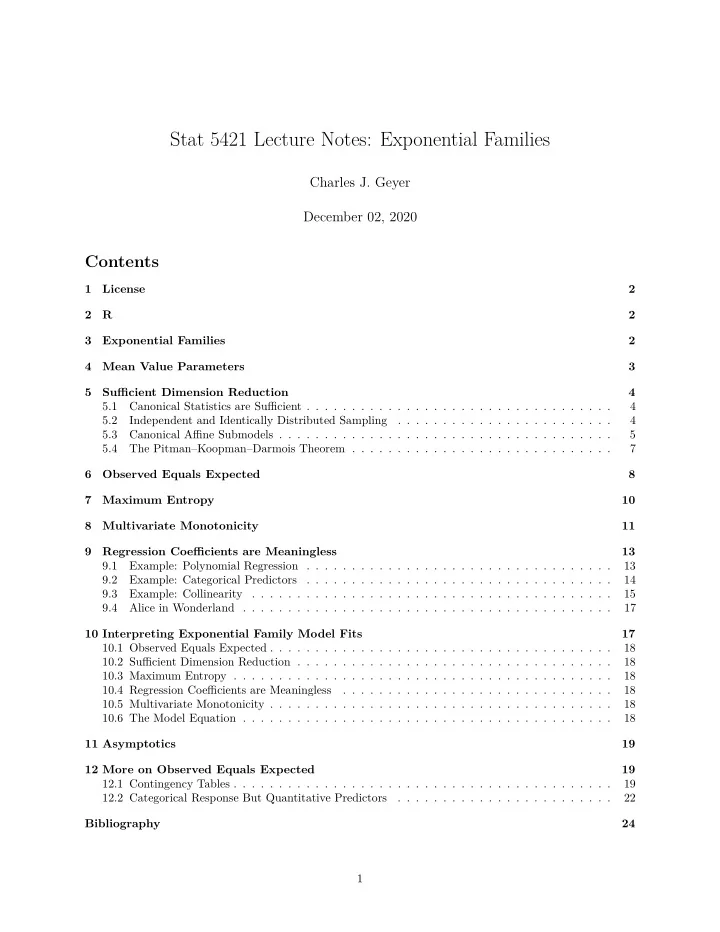
Stat 5421 Lecture Notes: Exponential Families Charles J. Geyer December 02, 2020 Contents 1 License 2 2 R 2 3 Exponential Families 2 4 Mean Value Parameters 3 5 Sufficient Dimension Reduction 4 5.1 Canonical Statistics are Sufficient . . . . . . . . . . . . . . . . . . . . . . . . . . . . . . . . . . 4 5.2 Independent and Identically Distributed Sampling . . . . . . . . . . . . . . . . . . . . . . . . 4 5.3 Canonical Affine Submodels . . . . . . . . . . . . . . . . . . . . . . . . . . . . . . . . . . . . . 5 5.4 The Pitman–Koopman–Darmois Theorem . . . . . . . . . . . . . . . . . . . . . . . . . . . . . 7 6 Observed Equals Expected 8 7 Maximum Entropy 10 8 Multivariate Monotonicity 11 9 Regression Coefficients are Meaningless 13 9.1 Example: Polynomial Regression . . . . . . . . . . . . . . . . . . . . . . . . . . . . . . . . . . 13 9.2 Example: Categorical Predictors . . . . . . . . . . . . . . . . . . . . . . . . . . . . . . . . . . 14 9.3 Example: Collinearity . . . . . . . . . . . . . . . . . . . . . . . . . . . . . . . . . . . . . . . . 15 9.4 Alice in Wonderland . . . . . . . . . . . . . . . . . . . . . . . . . . . . . . . . . . . . . . . . . 17 10 Interpreting Exponential Family Model Fits 17 10.1 Observed Equals Expected . . . . . . . . . . . . . . . . . . . . . . . . . . . . . . . . . . . . . . 18 10.2 Sufficient Dimension Reduction . . . . . . . . . . . . . . . . . . . . . . . . . . . . . . . . . . . 18 10.3 Maximum Entropy . . . . . . . . . . . . . . . . . . . . . . . . . . . . . . . . . . . . . . . . . . 18 10.4 Regression Coefficients are Meaningless . . . . . . . . . . . . . . . . . . . . . . . . . . . . . . 18 10.5 Multivariate Monotonicity . . . . . . . . . . . . . . . . . . . . . . . . . . . . . . . . . . . . . . 18 10.6 The Model Equation . . . . . . . . . . . . . . . . . . . . . . . . . . . . . . . . . . . . . . . . . 18 11 Asymptotics 19 12 More on Observed Equals Expected 19 12.1 Contingency Tables . . . . . . . . . . . . . . . . . . . . . . . . . . . . . . . . . . . . . . . . . . 19 12.2 Categorical Response But Quantitative Predictors . . . . . . . . . . . . . . . . . . . . . . . . 22 Bibliography 24 1

1 License This work is licensed under a Creative Commons Attribution-ShareAlike 4.0 International License (http: //creativecommons.org/licenses/by-sa/4.0/). 2 R • The version of R used to make this document is 4.0.3. • The version of the rmarkdown package used to make this document is 2.5. 3 Exponential Families We will use the following definition (Geyer, 2009). A statistical model is an exponential family of distributions if it has a log likelihood of the form l ( θ ) = � y, θ � − c ( θ ) (1) where • y is a vector-valued statistic, which is called the canonical statistic , • θ is a vector-valued parameter, which is called the canonical parameter , • c is a real-valued function, which is called the cumulant function , • and � · , · � denotes a bilinear form that places the vector space where y takes values and the vector space where θ takes values in duality. In equation (1) we have used the rule that additive terms in the log likelihood that do not contain the parameter may be dropped. Any such terms have been dropped in (1). You may object to the angle brackets notation as unfamiliar and not what you saw in some other class and i y i θ i or ( y, θ ) or y · θ or y T θ or θ T y or one of the latter with little t or prime prefer some notation like � for transpose. In your humble author’s opinion, the angle brackets are superior because they make it clear that � y, y � or � θ, θ � is always obviously wrong, whereas y T y or θ T θ or the same in any other notation is not obviously wrong. The angle brackets notation comes from functional analysis. Although we usually say “the” canonical statistic, “the” canonical parameter, and “the” cumulant function, these are not uniquely defined: • any one-to-one affine function of a canonical statistic vector is another canonical statistic vector, • any one-to-one affine function of a canonical parameter vector is another canonical parameter vector, and • any real-valued affine function plus a cumulant function is another cumulant function. (see Section 5.3 below for the definition of affine function). These possible changes of statistic, parameter, or cumulant function are not algebraically independent. Changes to one may require changes to the others to keep a log likelihood of the form (1) above. Usually no fuss is made about this nonuniqueness. One fixes a choice of canonical statistic, canonical parameter, and cumulant function and leaves it at that. The cumulant function may not be defined by (1) above on the whole vector space where θ takes values. In that case it can be extended to this whole vector space by 2

� e � y,θ − ψ � �� � c ( θ ) = c ( ψ ) + log E ψ (2) where θ varies while ψ is fixed at a possible canonical parameter value, and the expectation and hence c ( θ ) are assigned the value ∞ for θ such that the expectation does not exist. The family is full if its canonical parameter space is Θ = { θ : c ( θ ) < ∞ } (3) and a full family is regular if its canonical parameter space is an open subset of the vector space where θ takes values. Almost all exponential families used in real applications are full and regular. So-called curved exponential families (smooth non-affine submodels of full exponential families) are not full. Constrained exponential families (Geyer, 1991) are not full. A few exponential families used in spatial statistics are full but not regular (Geyer and Møller, 1994). Many people use “natural” everywhere this document uses “canonical”. In this we are following Barndorff- Nielsen (1978). Many people also use an older terminology that says a statistical model is in the exponential family, where we say a statistical model is an exponential family. Thus the older terminology says the exponential family is the collection of all of what the newer terminology calls exponential families. The older terminology names a useless mathematical object, a heterogeneous collection of statistical models not used in any application. The newer terminology names an important property of statistical models. If a statistical model is a regular full exponential family, then it has all of the properties discussed here. If a statistical model is an exponential family (not necessarily full or regular), then it has many of the properties discussed here. Presumably, that is the reason for the newer terminology. In this we are again following Barndorff-Nielsen (1978). 4 Mean Value Parameters The reason why the cumulant function has the name it has is because it is related to the cumulant generating function (CGF). A cumulant generating function is the logarithm of a moment generating function (MGF). Derivatives of an MGF evaluated at zero give moments. Derivatives of a CGF evaluated at zero give cumulants. Cumulants are polynomial functions of moments and vice versa. Using (2), the MGF for an exponential family with log likelihood (1) is given by M θ ( t ) = E θ ( e ty ) = e c ( θ + t ) − c ( θ ) provided this formula defines an MGF, which it does if and only if it is finite for t in a neighborhood of zero, which happens if and only if θ is in the interior of the full canonical parameter space (3). So the cumulant generating function is K θ ( t ) = c ( θ + t ) − c ( θ ) provided θ is in the interior of Θ. It is easy to see that derivatives of K θ evaluated at zero are derivatives of c evaluated at θ . So derivatives of c evaluated at θ are cumulants. We will be only interested in the first two cumulants 3