Solving MIPs A typical approach is use branch and bound search with - PowerPoint PPT Presentation

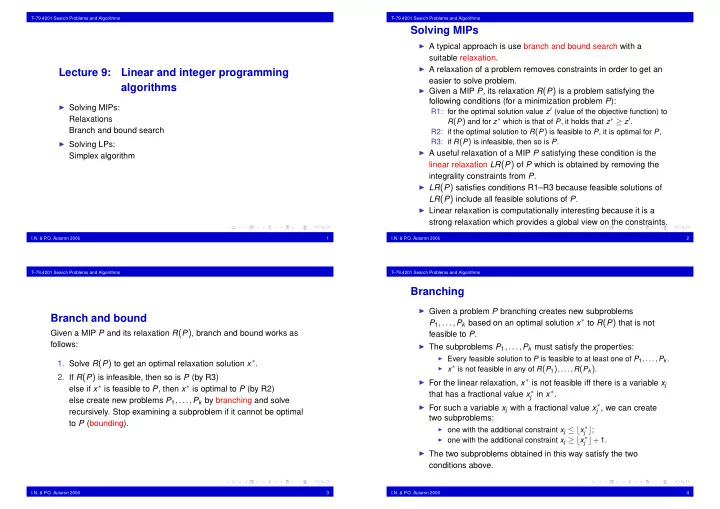
T–79.4201 Search Problems and Algorithms T–79.4201 Search Problems and Algorithms Solving MIPs ◮ A typical approach is use branch and bound search with a suitable relaxation. ◮ A relaxation of a problem removes constraints in order to get an Lecture 9: Linear and integer programming easier to solve problem. algorithms ◮ Given a MIP P , its relaxation R ( P ) is a problem satisfying the following conditions (for a minimization problem P ): ◮ Solving MIPs: R1: for the optimal solution value z ′ (value of the objective function) to R ( P ) and for z ∗ which is that of P , it holds that z ∗ ≥ z ′ . Relaxations R2: if the optimal solution to R ( P ) is feasible to P , it is optimal for P , Branch and bound search R3: if R ( P ) is infeasible, then so is P . ◮ Solving LPs: ◮ A useful relaxation of a MIP P satisfying these condition is the Simplex algorithm linear relaxation LR ( P ) of P which is obtained by removing the integrality constraints from P . ◮ LR ( P ) satisfies conditions R1–R3 because feasible solutions of LR ( P ) include all feasible solutions of P . ◮ Linear relaxation is computationally interesting because it is a strong relaxation which provides a global view on the constraints. I.N. & P .O. Autumn 2006 1 I.N. & P .O. Autumn 2006 2 T–79.4201 Search Problems and Algorithms T–79.4201 Search Problems and Algorithms Branching ◮ Given a problem P branching creates new subproblems Branch and bound P 1 ,..., P k based on an optimal solution x ∗ to R ( P ) that is not Given a MIP P and its relaxation R ( P ) , branch and bound works as feasible to P . follows: ◮ The subproblems P 1 ,..., P k must satisfy the properties: ◮ Every feasible solution to P is feasible to at least one of P 1 ,..., P k . 1. Solve R ( P ) to get an optimal relaxation solution x ∗ . ◮ x ∗ is not feasible in any of R ( P 1 ) ,..., R ( P k ) . 2. If R ( P ) is infeasible, then so is P (by R3) ◮ For the linear relaxation, x ∗ is not feasible iff there is a variable x j else if x ∗ is feasible to P , then x ∗ is optimal to P (by R2) that has a fractional value x ∗ j in x ∗ . else create new problems P 1 ,..., P k by branching and solve ◮ For such a variable x j with a fractional value x ∗ j , we can create recursively. Stop examining a subproblem if it cannot be optimal two subproblems: to P (bounding). ◮ one with the additional constraint x j ≤ ⌊ x ∗ j ⌋ ; ◮ one with the additional constraint x j ≥ ⌊ x ∗ j ⌋ + 1. ◮ The two subproblems obtained in this way satisfy the two conditions above. I.N. & P .O. Autumn 2006 3 I.N. & P .O. Autumn 2006 4

T–79.4201 Search Problems and Algorithms T–79.4201 Search Problems and Algorithms Improving Effectiveness Bounding ◮ Careful formulation ◮ Bounding also uses relaxation. ◮ Strong relaxations typically work well but are often bigger in size. ◮ Suppose we have generated a feasible solution to some ◮ Break symmetries. subproblem with solution value z ∗ . This could be optimal to a ◮ Multiple “big-M” values often lead to performance problems. subproblem but we do not yet know whether it is optimal to P . ◮ Deciding which formulation works better needs often experimentation. ◮ Then for each subproblem P i whose relaxation R ( P i ) has the ◮ Cutting plans optimal solution value z ′ i ≥ z ∗ , we can cease examining this These are constraints that are added to a relaxation to “cut off” subproblem (bounding). the optimal relaxation solution x ∗ . Often are problem specific but ◮ This is because by R1 z ∗ i ≥ z ′ i where z ∗ i is the optimal (minimum) there are also general techniques (e.g. Gomory cuts). solution value for P i and, hence, it is not possible to find a ◮ Special branching rules solution with a smaller solution value than z ∗ among the feasible solutions to P i . In many systems, for example, Special Ordered Sets are available. I.N. & P .O. Autumn 2006 5 I.N. & P .O. Autumn 2006 6 T–79.4201 Search Problems and Algorithms T–79.4201 Search Problems and Algorithms Simplex Method ◮ Assumes that the linear program is in standard form: Solving Linear Relaxation n ◮ Linear Relaxation of a MIP gives a linear program (LP) ∑ c i x i s.t. min ◮ There are a number of well-known techniques for solving LPs i = 1 n ◮ Simplex method ∑ a ij x j = b i , i = 1 ,..., m The oldest and most widely used method with very mature j = 1 implementation techniques. x j ≥ 0 , j = 1 ,..., n Worst-case time complexity exponential but seems to work extremely well in practice. ◮ The basic idea: start from a basic feasible solution and look at the ◮ Interior point methods adjacent ones. If an improvement in cost is possible by moving to A newer approach; polynomial time worst case time complexity; an adjacent solution, we do so. An optimal solution has been implementation techniques advancing found if no improvement is possible. ◮ Next, Simplex method is reviewed as an example. ◮ Next we briefly review the basic concepts needed: ◮ basic feasible solutions (bfs) ◮ move from one bfs to another (pivoting) ◮ the overall simplex algorithm I.N. & P .O. Autumn 2006 7 I.N. & P .O. Autumn 2006 8

T–79.4201 Search Problems and Algorithms T–79.4201 Search Problems and Algorithms Example Basic Feasible Solutions ◮ Consider the LP ◮ Assume an LP in standard form with m linear equations and n min 2 x 2 + x 4 + 5 x 7 variables x 1 ,..., x n , m < n . x 1 x 2 x 3 x 4 + + + = 4 ◮ A solution to the LP is an assignment of a real number to each x 1 x 5 + = 2 variable x i such that all equations are satisfied. x 3 x 6 + = 3 ◮ A solution safisfying the following condition is called a basic 3 x 2 x 3 x 7 + + = 6 solution: x 1 ,..., x 7 ≥ 0 ◮ n − m variables are set to 0 and ◮ the assignment for the other m variables (the basis) gives a ◮ For example, the basis ( x 4 , x 5 , x 6 , x 7 ) gives a basic feasible unique solution to the resulting set of m linear equations. solution x 0 = ( 0 , 0 , 0 , 4 , 2 , 3 , 6 ) because ◮ This means that a basic solution is obtained by choosing m x 4 = 4 , x 5 = 2 , x 6 = 3 , x 7 = 6 is the unique solution to the variable as the basis, setting the other n − m variables to zero resulting set of equations: and solving the resulting set of equations for the basic variables. x 4 + + + = 0 0 0 4 If there is a unique solution, this is gives a basic solution. x 5 + = 0 2 ◮ A basic feasible solution (bfs) is a basic solution such that every x 6 + = 0 3 variable is assigned a value ≥ 0. x 7 3 · 0 + + = 0 6 I.N. & P .O. Autumn 2006 9 I.N. & P .O. Autumn 2006 10 T–79.4201 Search Problems and Algorithms T–79.4201 Search Problems and Algorithms Moving from bfs to bfs Tableaux ◮ When moving from one bfs to another the idea is to remove one ◮ Pivoting is handled by keeping the set of equations diagonalized variable from the basis and replace it with another. This is called with respect to the basic variables. pivoting. ◮ This can be achieved using elementary row operations (Gaussian ◮ In Simplex this is organized as a manipulation of a tableau where, elimination): multiplying a row with a non-zero constant; adding a for instance, a set of equations row to another. 3 x 1 2 x 2 x 3 + + = Given a basis B = ( x 3 , x 4 , x 5 ) , we 1 Example. 5 x 1 x 2 x 3 x 4 + + + = 3 can transform the tableau to a di- Consider the set of equations 2 x 2 5 x 2 x 3 x 5 + + + = 4 agonalized form w.r.t. it by multi- plying Row 1 with -1 and adding x 1 x 2 x 3 x 4 x 5 is represented as it to Rows 2 and 3: 1 3 2 1 0 0 x 1 x 2 x 3 x 4 x 5 3 5 1 1 1 0 x 1 x 2 x 3 x 4 x 5 4 2 5 1 0 1 1 3 2 1 0 0 1 3 2 1 0 0 3 5 1 1 1 0 − 1 2 2 0 1 0 4 2 5 1 0 1 − 1 3 3 0 0 1 I.N. & P .O. Autumn 2006 11 I.N. & P .O. Autumn 2006 12