Scheduling and Timetabling Integer linear programming models Marjan - PowerPoint PPT Presentation
Scheduling and Timetabling Integer linear programming models Marjan van den Akker 1 I ntro. Marjan van den Akker Lecturer/research Algorithms and Complexity group: Coordination Software- and Gameproject Master courses :
Scheduling and Timetabling Integer linear programming models Marjan van den Akker 1
I ntro……. Marjan van den Akker Lecturer/research Algorithms and Complexity group: Coordination Software- and Gameproject Master courses : Algorithms for decision support (COSC), Advanced Linear Programming (Mastermath) Research on planning/scheduling algorithms: Public transportation Sustainable energy systems integer linear programming and local search simulation 2 4/24/2018
Contents Integer linear programming is well-known modelling and solution technique First, linear programming Modelling integer linear programming problems This is material from the course Algorithms for Decision Support NB: we will work a lot on the blackboard. You are strongly advised to take notes. A beautiful reader is available at http://www.cs.uu.nl/docs/vakken/mads/LectureNotesILP.pdf 3 ADS, ILP 1
Exam ple: Ajax Three types of computers: Alpha, Beta, and Gamma. Net profit: $350,- per Alpha, $470,- per Beta, and $610,- per Gamma. Every computer can be sold at the given profit. Testing: Alpha and Beta computers on the A-line, Gamma computers on the C-line. Testing takes 1 hour per computer. Capacity A-line: 120 hours; capacity C-line: 80 hours. Required labor: 10 hours per Alpha, 15 hours per Beta, and 20 hours per Gamma. Total amount of labor available: 2000 hours. 4 4 SCM, chapter 3
Exam ple: Ajax Decision variables: MA number of alpha’s produced, etc Objective function max Z 350 MA 470 MB 610 MC subject to MA MB 120 (A line) Constraints MC 48 ( C line ) 10 MA 15 MB 20 MC 2000 ( labor ) MA , MB , MC 0 5 5 SCM, chapter 3
Linear program m ing Min c T x s.t. Ax ≤ b x ≥ 0 With � ∈ � � , � ∈ ℚ � , A ∈ ℚ ��� , and � ∈ ℚ � 6 ADS, ILP 1
LP:Geom etric x 2 5 3 (4,4) x 3 x 1 2 x 1 x 2 1 2 1 x 1 0 2 x max x 1 2 x 2 0 1 2 3 ADS, ILP 1 7
The sim plex m ethod Example dictionaries 8 ADS, ILP 1
9 ADS, ILP 1
10 ADS, ILP 1
11 ADS, ILP 1
12 ADS, ILP 1
13 ADS, ILP 1
14 ADS, ILP 1
15 ADS, ILP 1
Solution options A linear programming problem can be infeasible Example: max 6� � � 4� � � � � � � � 3, 2� � � 2� � � 8, � � , � � � 0� be unbounded Example: max 6� � � 4� � � � � � � � 3, 2� � � 2� � � 8, � � , � � � 0� for any � � 0 we have that � � � �, � � � � is feasible have a bounded optimum 16 ADS, ILP 1
Solution m ethod for linear program m ing Seems not too hard to implement. But, for larger Simplex method problems you run into Slower than polynomial numerical problems. Use a Practical standard solver (Gurobi, Ellipsoid method CPLEX, GLPK) Polynomial (Khachian, 1979) Not practical Interior points methods Polynomial (Karmakar, 1984) Outperforms Simplex for very large instances LP P 17 ADS, ILP 1
Knapsack problem Knapsack with volume 15 What should you take with you to maximize utility? Item 1:paper 2:book 3:bread 4:smart 5:water -phone Utility 8 12 7 15 12 Volume 4 8 5 2 6 ADS, ILP 1 18 18
Knapsack problem ( 2 ) x 1 = 1 if item 1 is selected, 0 otherwise, x 2 , …… max z= 8 x 1 + 12 x 2 + 7 x 3 + 15 x 4 + 12 x 5 subject to 4 x 1 + 8 x 2 + 5 x 3 + 2 x 4 + 6 x 5 ≤ 15 x 1 , x 2 , x 3 , x 4 , x 5 Є {0,1} 19 ADS, ILP 1
( Mixed) I nteger linear program m ing Min c T x + d T y s.t. Ax + By ≤ b x,y ≥ 0 x integral (or binary) Extension of LP: Good news: more possibilities for modelling Bad news: larger solution times 20 ADS, ILP 1
( Mixed) I nteger linear program LP-relaxation Min c T x Min c T x s.t. Ax + By ≤ b s.t. Ax + By ≤ b x,y ≥ 0 x,y ≥ 0 x integral (or binary) Lower bound (or upper bound in case of maximization) 21 ADS, ILP 1
22 ADS, ILP 1
Modeling Decision variables Objective function Constraints 23 ADS, ILP 1
Assignm ent problem n persons, n jobs. Each person can do at most one job Each job has to be executed C ij cost if person i performs job j We want to minimize cost 24 ADS, ILP 1
Maxim um independent set Given a graph G=(V,E) V: nodes E: edges An independent set I is a set of nodes, such that every edge has at most one nodes in I, i.e., no pair of nodes in I is connected. What is the maximum number of nodes in an independent set? 25 ADS, ILP 1
Facility location Possible locations: n Customers: m 26 ADS, ILP 1
Capacitated facility location Data: m customers, Customer demand: D i n possible locations of depots (facilities) c ij unit cost of serving customer i by depot j Capacity depot: C j Fixed cost for opening depot DC: F j Which depots are opened and which customer is served by which depot? 27 ADS, ILP 1
Uncapacitated facility location Data: m customers, n possible locations of depot Each customer is assigned to one depot d ij cost of serving customer i by depot j Fixed cost for opening depot DC: F j Which depots are opened and which customer is served by which depot? 28 ADS, ILP 1
Uncapacitated facility location Two models FL and AFL Same optimal value Z IP for ILP Set of feasible solutions for LP-relaxation satisfy: � �� ⊆ � ��� Set of optimal values satisfy: � ��� � � �� � � �� The LP-relaxation of FL gives a stronger bound 29 ADS, ILP 1
Single m achine scheduling exam ple n jobs, 1 machine Job j requires uninterrupted processing time P j Job j has release date r j Machine can process at most one job at a time We want to minimize the weighted sum of the completion times This is going to be denoted by 30 ADS, ILP 1
Recommend
More recommend
Explore More Topics
Stay informed with curated content and fresh updates.
