Recent Progresses on the Simplex Method Yinyu Ye - PowerPoint PPT Presentation
Recent Progresses on the Simplex Method Yinyu Ye www.stanford.edu/~yyye K.T. Li Professor of Engineering Stanford University and International Center of Management Science and Engineering Nanjing University November 2013 Yinyu Ye Outlines
Recent Progresses on the Simplex Method Yinyu Ye www.stanford.edu/~yyye K.T. Li Professor of Engineering Stanford University and International Center of Management Science and Engineering Nanjing University November 2013 Yinyu Ye
Outlines • Linear Programming (LP) and the Simplex Method • Markov Decision Process (MDP) and its LP Formulation • Simplex and policy-iteration methods for MDP and Zero-Sum Game with fixed discounts • Simplex method for general non-degenerate LP (including the unbounded case) • Open Problems November 2013 Yinyu Ye
Linear Programming started… November 2013 Yinyu Ye
… with the simplex method November 2013 Yinyu Ye
LP Model in Dimension d max c c c x x x + + + max c x c x c x + + + 1 1 2 2 n n 1 1 2 2 d d s.t. s.t. a a a b x x x ≤ + + + a x a x a x ≤ b + + + 1 2 n 11 12 1n 1 11 1 12 2 1 d d 1 a x a x a x ≤ b + + + a x a x a x ≤ b + + + 21 1 22 2 2n n 2 21 1 22 2 2 d d 2 a x a x a x ≤ b + + + a x a x a x b ≤ + + + m1 1 m2 2 mn n m n 1 1 n 2 2 nd d n x ≥ x ≥ x ≥ 0 , 0 , , 0 1 2 n The feasible region is a polyhedron defined by n inequalities in d dimensions. November 2013 Yinyu Ye
LP Geometry and Theorems • Optimize a linear objective function over a convex polyhedron, and there is always a vertex optimal solution. November 2013 Yinyu Ye
The Simplex Method • Start with any vertex, and move to an adjacent vertex with an improved objective value. Continue this process till no improvement. November 2013 Yinyu Ye
Pivoting rules … • The simplex method is governed by a pivot rule, i.e. a method of choosing adjacent vertices with a better objective function value. • Dantzig's original greedy pivot rule. • The lowest index pivot rule. • The random edge pivot rule chooses, from among all improving pivoting steps (or edges) from the current basic feasible solution (or vertex), one uniformly at random. November 2013 Yinyu Ye
Markov Decision Process • Markov decision process provides a mathematical framework for modeling sequential decision- making in situations where outcomes are partly random and partly under the control of a decision maker. • MDPs are useful for studying a wide range of optimization problems solved via dynamic programming, where it was known at least as early as the 1950s (cf. Shapley 1953, Bellman 1957). • Modern applications include dynamic planning, reinforcement learning, social networking, and almost all other dynamic/sequential decision making problems in Mathematical, Physical, Management, Economics, and Social Sciences. November 2013 Yinyu Ye
States and Actions • At each time step, the process is in some state i = 1 , ...,m , and the decision maker chooses an action j ∈ A i that is available for state i, say of total n actions. • The process responds at the next time step by randomly moving into a new state i’ , and giving the decision maker an immediate corresponding cost c j . • The probability that the process enters i’ as its new state is influenced by the chosen action j . Specifically, it is given by the state transition probability distribution P j . • But given action j , the probability is conditionally independent of all previous states and actions; in other words, the state transitions of an MDP possess the Markov property. November 2013 Yinyu Ye
A Simple MDP Problem I November 2013 Yinyu Ye
Policy and Discount Factor • A policy of MDP is a set function π = { j 1 , j 2 , ・ ・ ・ , j m } that specifies one action j i ∈ A i that the decision maker will choose for each state i . • The MDP is to find an optimal (stationary) policy to minimize the expected discounted sum over an infinite horizon with a discount factor 0 ≤ γ < 1. • One can obtain an LP that models the MDP problem in such a way that there is a one-to-one correspondence between policies of the MDP and basic feasible solutions of the (dual) LP, and between improving switches and improving pivots. de Ghellinck (1960), D’Epenoux (1960) and Manne (1960) November 2013 Yinyu Ye
Cost-to-Go-Values 1 1 1 1 1 3/4 1/2 7/8 0 Chosen actions in Red November 2013 Yinyu Ye
Cost-to-Go values and LP formulation • Let y ∈ R m represent the expected present cost- to-go values of the m states, respectively, for a given policy. Then, the cost-to-go vector of the optimal policy is a Fixed Point of = + ∈ ∀ T y min{ c p y , j A }, i , γ i j j i = + ∈ ∀ T j arg min{ c p y , j A }, i . γ i j j i • Such a fixed point computation can be formulated as an LP m ∑ max y i = i 1 ≤ + ∀ ∈ ∀ T s.t. y c p y , j A ; i . γ i j j i November 2013 Yinyu Ye
The dual of the MDP-LP n ∑ min c x j j = i 1 n ∑ − γ = ∀ s.t. ( e p ) x 1 , i , ij ij j = j 1 ≥ ∀ x 0 , j . j where e ij =1 if j ∈ A i and 0 otherwise. Dual variable x j represents the expected action flow or visit-frequency, that is, the expected present value of the number of times action j is used. November 2013 Yinyu Ye
Greedy Simplex Rule Chosen actions in Red November 2013 Yinyu Ye
Lowest-Index Simplex Rule Chosen actions in Red November 2013 Yinyu Ye
Policy Iteration Rule (Howard 1960) Chosen actions in Red November 2013 Yinyu Ye
Exponentially bad examples • Klee and Minty (1972) showed that Dantzig's original greedy pivot rule may require exponentially many steps for a LP example. • Melekopoglou and Condon (1990) showed that the simplex method with the smallest index pivot rule needs an exponential number of iterations for a MDP example regardless of discount factors. • Fearnley (2010) showed that the policy-iteration method needs an exponential number of iterations for a undiscounted finite-horizon MDP example. • Friedmann, Hansen and Zwick (2011) gave an undiscounted MDP example that the random edge pivot rule needs sub-exponentially many steps. November 2013 Yinyu Ye
Any Good News? • In practice, the policy-iteration method, including the simplex method with greedy pivot rule, has been remarkably successful and shown to be most effective and widely used. • Any good news in theory? November 2013 Yinyu Ye
Bound on the simplex/policy methods • Y (2011): The classic simplex and policy iteration methods, with the greedy pivoting rule, terminate in no more than 2 mn m ( 1 ) log − γ − γ 1 pivot steps, where n is the total number of actions in an m -state MDP with discount factor γ . • This is a strongly polynomial-time upper bound when γ is bounded above by a constant less than one. November 2013 Yinyu Ye
Roadmap of proof • Define a combinatorial event that cannot repeats more than n times. More precisely, at any step of the pivot process, there exists a non-optimal action j that will never re-enter future policies or bases after 2 m m ( 1 ) log − γ − γ 1 pivot steps • There are at most (n - m) such non-optimal action to eliminate from appearance in any future policies generated by the simplex or policy-iteration method. • The proof relies on the duality, the reduced-cost vector at the current policy and the optimal reduced- cost vector to provide a lower and upper bound for a non-optimal action when the greedy rule is used. November 2013 Yinyu Ye
Improvement and extension Hansen, Miltersen and Zwick (2011): • For the policy iteration method terminates in no more 2 n m ( 1 ) log − γ − γ 1 steps. • The simplex and policy iteration methods, with the greedy pivoting rule, are strongly polynomial- time algorithms for Turn-Based Two-Person Zero-Sum Stochastic Game with any fixed discount factor, which problem cannot even be formulated as an LP. November 2013 Yinyu Ye
A Turn-Based Zero-Sum Game November 2013 Yinyu Ye
Deterministic MDP with discounts Distribution vector p j ∈ R m contains exactly one 1 and 0 everywhere else = + ∈ ∀ T y min{ c p y , j A }, i , γ i j j j i = + ∈ ∀ T j arg min{ c p y , j A }, i . γ i j j j i m ∑ max y i = i 1 ≤ + ∀ ∈ ∀ T s.t. y c p y , j A ; i . γ i j j j i It has uniform discounts if all γ j are identical. November 2013 Yinyu Ye
The dual resembles a generalized flow n ∑ min c x j j = i 1 n ∑ − γ = ∀ s.t. ( e p ) x 1 , i , ij j ij j = j 1 ≥ ∀ x 0 , j . j where e ij =1 if j ∈ A i and 0 otherwise. Dual variable x j represents the expected action flow or frequency, that is, the expected present value of the number of times action j is chosen. November 2013 Yinyu Ye
Recommend
More recommend
Explore More Topics
Stay informed with curated content and fresh updates.







![CS156: The Calculus of F [ x 1 , . . . , x n ] or x 1 , . . . , x n . F [ x 1 , . . . , x n ]](https://c.sambuz.com/1006519/cs156-the-calculus-of-s.webp)
