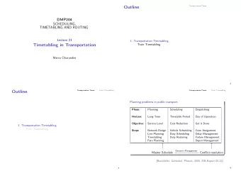
Timetabling and Scheduling Marco Chiarandini Outline 1. - - PowerPoint PPT Presentation

LOCAL SEARCH METHODS

APPLICATIONS AND ENGINEERING

Lecture 8

Timetabling and Scheduling

Marco Chiarandini

Outline

• 1. Timetabling

Educational Timetabling

Solution Methods for the Course Timetabling An Example

Workforce Scheduling

• 2. Scheduling

Problem Classification Single Machine Scheduling Flow Shop Scheduling

Local Search Methods: Applications and Engineering 2

Outline

• 1. Timetabling
• 2. Scheduling

The Timetabling Activity

Assignment of events to a limited number of time periods and locations subject to constraints

Types of timetabling

◮ Class Timetabling ◮ Exams Timetabling ◮ Courses Timetabling ◮ Employee Timetabling ◮ Crew Scheduling ◮ Crew Rostering ◮ Nurse Timetabling ◮ Transport Timetabling, ◮ Sport Timetabling, ◮ Communication Timetabling

In general timetabling varies from institution to institution in terms of constraints, requirements and their density

Two Types of Constraints:

◮ Hard constraints H = {H1, . . . , Hn}: their violation is not allowed ◮ Soft constraints Σ = {S1, . . . , Sm}: their violation should be minimized

Local Search Methods: Applications and Engineering 4

School (class/teacher, parent/teacher) model

A class is a set of students who follow exactly the same program. Each class has a dedicated room. Input: a set of classes C = {c1, . . . , cm}, a set of teachers T = {t1, . . . , tn} and r periods P1, . . . , Pr. A requirement matrix Rm×n where rij is the number of lectures given by teacher tj to class ci. Output: An assignment of lectures to periods such that no teacher is involved in more than one lecture at a time. Graph model: Edge Coloring of a bipartite multigraph G = (C, T, R). Solvable in polynomial time by solving sequences of maximal matchings or network flows problems.

Further constraints:

◮ Weekly schedule, a period represents

a set of periods, e.g., the same period in each day of a week

◮ Maximum number of lectures in

which C and T can be involved in a day (bounded edge coloring)

◮ Pre-assignments ◮ Unavailabilities ◮ Daily load is spread, balanced ◮ Specific day off for a teacher ◮ Desirability of assignment tj to class

ci in pk

Exam Model

There is one exam for each subject. Exams with common students are conflicting exams. There are constraints that tend to separate consecutive exams for students. The number of periods is not a strict constrain. Input: A set of courses C = {c1, . . . , cm} and one exam for each course. A set of groups of exams S = {S1, . . . , Sp} such that in each Sl there are students that take exams in Sl. A set of periods P1, . . . , Pr and a set of rooms R = {R1, . . . , Rr} available at each period. Output: An assignment of each exam ci to some period in such a way that no student is required to take more than one exam at a time. Graph model: Vertex Coloring of a graph in which each exam ci is a vertex and each conflict an edge.

Further constraints:

◮ Avoid that students have exams in consecutive periods ◮ Pre-assignments ◮ Unavailabilities ◮ Minimize the number of periods ◮ Room assignment with more than one exam per room

Course Model

Courses are made of lectures which have common students. Professors teach

• nly one course. Assignment of rooms according to availability and suitability.

Input: A set of courses C = {C1, . . . , Cn} each consisting of li lectures, Ci = {L1, . . . , Lli}. A set of curricula S = {S1, . . . Sr} which are groups of courses with common students. A set of periods P1, . . . , Pr and a set of rooms R = {R1, . . . , Rr} available per each period. Output: An assignment of each lecture Li to some period in such a way that no student is required it take more than one lecture at a time. Graph model: Vertex Coloring each lecture Li constitutes a vertex and each conflict an edge.

An Example of Course Timetabling

Local Search Methods: Applications and Engineering 8

Typical Constraints in Course Timetabling

Hard Constraints:

◮ All required lectures must be scheduled ◮ Only one lecture is scheduled in one room at any period ◮ Lectures of the same curriculum must be scheduled in different periods ◮ Unavailabilities of professors in some periods ◮ Unavailabilities of rooms for courses due to lack of suitable facilities ◮ Pre-assignments of lectures in a determined room and period

Soft Constraints:

◮ Professors’ preferences for teaching in some periods ◮ Preferences room-courses ◮ Room capacity must match the number of students attending a lecture ◮ Minimal number of working days (ex, a course with 5 lectures of 2 hours must

be held in a minimum of 4 days)

◮ Intervals limiting the number of lectures per student in a day (ex, 2-3) ◮ Preferences on the minimal separation between consecutive lectures (ex, due

to logistic constraints)

◮ Limit on the number of consecutive lectures ◮ Lectures of a same course must be scheduled in the same room

In Practice

A timetabling system consists of:

◮ Solver (written in a fast language, i.e., C, C++) and various interfaces

to handle the input and output

◮ Input and Output management (textual files or output in HTML format) ◮ Declaration of constraints (professors’ preferences may be inserted

directly through a web interface and stored in the information system of the University) The whole timetabling process:

• 1. Collect data from the information system
• 2. Execute a few runs of the Solver starting from different solutions

selecting the timetable of minimal cost. The whole computation time should not be longer than one night. This becomes a “draft” timetable.

• 3. The draft is shown to the professors who can require adjustments. The

adjustments are obtained by defining new constraints to pass to the Solver.

• 4. Post-optimization of the “draft” timetable using the new constraints
• 5. The timetable can be further modified manually by using the Solver to

validate the new timetables.

Local Search Methods: Applications and Engineering 10

Solution Approaches

◮ Typically solved in two (or more) phases: first a feasible solution

satisfying all hard constraints is found and then the soft constraints are considered. Issue: exiting or not from feasibility?

◮ Handling the soft constraints gives rise to a multi-objective problem.

Three approaches: Combine objectives: combination of penalties into a single value by means of weights Goal programming: assign priorities and goal values to the objectives and optimize one objective at a time while imposing constraints on the others. Pareto-based: the whole Pareto-frontier of trade off solutions is determined

◮ The classroom assignment sub-problem can be solved efficiently if each

period is considered independently

Local Search Methods: Applications and Engineering 11

Search Space Timetabling representation

◮ Graph coloring: it does not comprises the assignment of rooms ◮ Matrix representation: it comprises the assignment of rooms

Rooms Periods P1 P2 Pi Pj P45 R1 −1 L4 · · · L10 · · · L14 · · · −1 R2 L1 L5 · · · L11 · · · L15 · · · −1 R3 L2 L6 · · · L12 · · · −1 · · · −1 . . . . . . . . . . . . . . . Rr L3 L7 · · · L13 L16 · · · −1

Two search approaches:

◮ Complete assignment of lectures (requirement constraints satisfied) ◮ Partial assignment of lectures (requirement constraints not satisfied)

Local Search Methods: Applications and Engineering 12

Construction Heuristics

They are inspired by heuristics for GCP and consist of two main passages:

◮ Deciding the next lecture to schedule ◮ Deciding a place in the assignment matrix for the selected lecture

For example:

Step 1. Initialize the set b L of all unscheduled events with b L = L. Step 2. Choose a lecture Li ∈ b L according to a heuristic rule. Step 3. Let b X be the set of all positions for Li in the assignment matrix with minimal violations of the hard constraints H. Step 4. Let ¯ X ⊆ b X be the subset of positions of b X with minimal violations of the soft constraints Σ is minimized. Step 5. Choose an assignment for Li in ¯ X according to a heuristic rule. Update information. Step 6. Remove Li from b L, and go to step 2 until b L is not empty.

Local Search Methods: Applications and Engineering 13

Neighborhood Structures for Perturbative Search

T1 T2 T3 T4 T5 T6 T7 T8 T9 T10 T11 T12 T13 T14 T15 T16 T17 T18 T19 T20 T21 T22 T23 T24 T25 T26 T27 R10 382 1 56 362 45 247 392 85 389 384 17 394 200 294 273 391 180 42 157 388 397 331 131 363 383 R9 396 144 173 78 25 183 387 337 240 132 328 212 370 308 336 244 126 14 231 51 342 136 93 129 266 393 155 R8 256 32 147 270 289 130 48 282 116 251 307 44 260 79 296 242 150 81 353 158 293 338 218 161 R7 228 31 107 371 30 355 46 227 246 271 182 313 224 128 89 258 356 343 280 35 109 306 43 83 11 154 R6 322 225 352 28 168 72 49 69 12 92 38 373 390 164 135 121 268 115 75 87 140 165 104 137 133 385 346 R5 324 291 309 339 267 283 269 170 299 311 34 65 216 275 199 26 27 327 33 39 285 R4 181 160 90 82 193 206 156 152 341 179 171 226 4 348 127 365 213 80 R3 263 71 186 67 222 288 99 24 237 232 253 117 195 203 102 207 287 290 146 286 358 303 277 R2 360 345 2 153 354 91 61 319 349 278 86 204 316 220 323 176 314 7 108 50 312 235 330 R1 187 239 378 66 380 53 208 279 300 350 211 375 254 366 369 223 163 298 118 368 234 97 329 274 58 Monday Tuesday Wednesday T1 T2 T3 T4 T5 T6 T7 T8 T9 T10 T11 T12 T13 T14 T15 T16 T17 T18 T19 T20 T21 T22 T23 T24 T25 T26 T27 R10 382 1 56 362 45 247 392 85 389 384 17 394 200 294 273 391 180 42 157 388 397 331 131 363 383 R9 396 144 173 78 25 183 387 337 240 132 328 212 370 308 336 244 126 14 231 51 342 136 93 129 266 393 155 R8 256 32 147 270 289 130 48 282 116 251 307 44 260 79 296 242 150 81 353 158 293 338 218 161 R7 228 31 107 371 30 355 46 227 246 271 182 313 224 128 89 258 356 343 280 35 109 306 43 83 11 154 R6 322 225 352 28 168 72 49 69 12 92 38 373 390 164 135 121 268 115 75 87 140 165 104 137 133 385 346 R5 324 291 309 339 267 283 269 170 299 311 34 65 216 275 199 26 27 327 33 39 285 R4 181 160 90 82 193 206 156 152 341 179 171 226 4 348 127 365 213 80 R3 263 71 186 67 222 288 99 24 237 232 253 117 195 203 102 207 287 290 146 286 358 303 277 R2 360 345 2 153 354 91 61 319 349 278 86 204 316 220 323 176 314 7 108 50 312 235 330 R1 187 239 378 66 380 53 208 279 300 350 211 375 254 366 369 223 163 298 118 368 234 97 329 274 58

◮ N1: One-Exchange ◮ N2: Two-Exchange ◮ N3: Period Interchange ◮ N4: Kempe Chain Interchange

Local Search Methods: Applications and Engineering 14

Local Search Methods

Basic components Construction Iterative Improvement Heuristics Metaheuristics Assemblage Testable units Testable units Testable units

heuristics Tabu Search Simulated Anneling Iterated Local Search Iterated Greedy Ant Colony Optimization Evolutionary Algorithm Solving the global problem Hard constraints, Soft Constraints Graph Coloring, Bipartite Matching, Solving sub−problems neighborhood structures Portfolio of Portfolio of configurations algorithm

Local Search Methods: Applications and Engineering 15

An Example in Practice Course Timetabling at the University of Edinburgh

Find an assignment of lectures to periods and rooms which is Feasible

rooms are only used by one lecture at a time, each lecture is assigned to a suitable room, no student has to attend more than one lecture at once; 9 = ; Hard Constraints

and Good

not more than two lectures in a row for a student, unpopular periods avoided (last in a day), students do not have one single lecture in a day. 9 = ; Soft Constraints

Local Search Methods: Applications and Engineering 16

Algorithm Flowchart

• It. Improvement

Kempe−chains

• It. Improvement

timeslot swap Simulated Annealing

• ne−ex and swap

with Matching Tabu Search

• ne−ex

Preprocessing Timetable Construct

• ne−ex and swap
• It. Improvement

5 loops?

• It. Improvement
• ne−ex
• ne−ex and swap
• It. Improvement
• It. Improvement
• ne−ex and swap

with matching improvement? any Soft Constraints Optimizer no Hard Constraints Solver yes feasible? Select the best from Archive Add into Archive no yes

• It. Improvement
• ne−ex

yes no yes no heuristics all used?

Local Search Methods: Applications and Engineering 17

Workforce Scheduling Classification in terms of application areas:

◮ Crew Scheduling (in transportation and logistic) ◮ Nurse Scheduling (in health/social system) ◮ Employee Scheduling (in production and service)

Time horizon of the schedule, yielding typically decomposed problems:

◮ long term: “staffing” based on demand estimations ◮ short term: staff rostering ◮ real-time: reallocation

Rostering: the placing, subject to constraints, of persons into slots of a

• pattern. Often the resources will rotate through a roster of a determined

duration (eg, one week).

Local Search Methods: Applications and Engineering 18

The Terminology of Nurse Rostering

◮ Planning Period: the time (usually 4 weeks) over which the schedule

take place

◮ Skill Category: qualification of the staff to accomplish a certain task ◮ Shift Type: well defined start and end time ◮ Coverage Constraints (= personnel demand/requirements): express the

number of persons needed for every skill category and for every shift

◮ Time Related Constraints: restrictions or preferences on personal

schedules

◮ Work Regulations: time related constraints due to the contract the

personnel member has with the hospital

Local Search Methods: Applications and Engineering 19

A List of Characteristics of Nurse Rostering

◮ Coverage and time related constraints considered as hard and/or soft constraints ◮ Flexibility of setting and defining problem parameters

Fixed// Adaptable// User definable

◮ Cyclical and non-cyclical approaches ◮ Approaches for tackling coverage constraints

Under-staffing Allowed/Not allowed// Over-staffing Allowed/Not allowed

◮ Number of skill categories and substitutability

Skill categories scheduled separately// Hierarchical substitutability: people with a higher skill category can replace the lower// User definable substitutability

◮ Flexibility in setting and defining work regulations

Identical work regulations for all people// Mixed workforce: Full time and half time personnel// User definable work regulations// Float personnel

◮ Different definitions of coverage constraints

Constant// Weekdays-weekends// Fluctuating: the coverage constraints vary over the planning period

◮ Flexibility of defining shift types

One single shift or no shifts defined: days// Three different shifts: usually referred to as Morning// Late and Night shift// Defined length: the intervals cannot be set by the users// User definable shifts: the number of different shifts// their start and end times and their length are set by the users

◮ Possible planning periods

4 days// 1,2,3 weeks// 1 month

Local Search Methods: Applications and Engineering 20

◮ Staff size

User definable fixed number// To be minimized

◮ Time related constraints: Capacity

Max number of assignments// Overtime// Max number of assignments to a particular Shift Type// Max number of shifts per week

◮ Time related constraints: Personal preferences

Days off// Shifts off// Days on// Shift on// Shift patterns// Shift sequences

◮ Time related constraints: Consecutiveness constraints

Max/min/fixed number of consecutive (free) days// Patterns// Free days after night shifts// No night shift before day off// Time between assignments// Consecutive shifts// Sequences of shift types// Mixture of day-night shifts per Week

◮ Time related constraints: Balance the workload ◮ Time related constraints: Weekends

Complete weekends and extended weekends// Compensation of weekend work// Number of consecutive weekends

◮ Time related constraints: Others

Preference days/nights// Changes in shifts on consecutive days// Maximum consecutive on/off/on patterns// People working together or not

◮ Objectives

Minimize: violations of time related constraints// violations of coverage constraints// violations of coverage and time related constraints// number of employees// personnel cost// non-negative ’under’ coverage// uneven distribution of shortages and surpluses over weekdays// deviation between scheduled nurses and demand // deviation between scheduled people and the total work capacity from the work regulations

Local Search Methods: Applications and Engineering 21

Perturbative Search Roster representation

Personnel Shifts Monday Tuesday · · · Early Day Night Early Day Night · · · P1 −− T1 −− −− T3 −− · · · P2 T1 −− −− T1 −− −− · · · P3 T2 −− −− −− −− T3 · · · . . . . . . . . . . . . . . . . . . . . . . . . Pr T3 −− −− T3 −− T1 · · ·

Neighborhood Structure

◮ 1-exchange within shifts ◮ 2-exchange within shifts ◮ insert/remove ◮ focused on specific

constraints

Local Search Methods: Applications and Engineering 22

Issues of Real Timetabling

◮ Fully address the needs and requirements of the real situation ◮ Generalized satisfaction: enterprise / employee ◮ Construction of the evaluation function, ie, in presence of conflicting

• bjectives

◮ Robustness and flexibility, ie, minimizing the number of necessary real

time changes consequent to unforeseen circumstances

◮ Maximize human/computer interaction ◮ Algorithm parameters hidden to the administrator ◮ Solution method hybridization ◮ Inter-disciplinarity: administration, management, psychology and

software engineering Definition Conflicting constraints

Local Search Methods: Applications and Engineering 23

Outline

• 1. Timetabling
• 2. Scheduling

Problem Definition Problem Definition

Given a set of jobs J = {J1, . . . , Jn} that have to be processed by a set of machines M = {M1, . . . , Mm} find a schedule, i.e., a mapping of jobs to machines and processing times subject to feasibility and optimization constraints.

Local Search Methods: Applications and Engineering 25

Problem Classification Machine Environment α1α2|β1β2β3β4|γ1γ2

◮ single machine/multi-machine (1/m) ◮ parallel machines: identical (P), uniform (Q), unrelated (R) ◮ Flow Shop (F), Open Shop (O), Job Shop and Group Shop (J)

Job Characteristics α1α2|β1β2β3β4|γ1γ2

◮ single-stage/multi-stage Ji = {oi1, . . . , oim(i)} ◮ processing times of jobs or operations machine dependent/independent ◮ release ri and due dates di associated with job Ji ◮ precedence constraints pij between jobs or operations ◮ weights wi associated with Ji ◮ setup times tij for jobs Ji, Jj (machine dep/indep)

Local Search Methods: Applications and Engineering 26

Objective α1α2|β1β2β3β4|γ1γ2

Measures:

◮ Completion time Ci for job Ji ◮ Lateness Li = Ci − di ◮ Tardiness Ti = max{Ci − di, 0} ◮ Earliness Ei = max{di − Ci, 0}

Typically, Minimize:

◮ maximum completion Cmax = makespan ◮ wi · Ci total completion time ◮ wi · Ti total tardiness

Regular objective functions vs irregular

Local Search Methods: Applications and Engineering 27

Single Machine Problems

◮ 1|dj|Lmax, 1|dj|Tmax (Maximum Lateness/Tardiness) solved exactly by

greedy earliest due date

◮ 1|dj|L Ti up to 500 jobs feasible exactly ◮ 1|dj|L wiTi up to 100 jobs feasible exactly

Local Search Methods: Applications and Engineering 28

Flow Shop Problems Characteristics:

◮ Multi-stage, Multi-machine ◮ The order in which the jobs pass through the machines is the same for

all jobs

◮ Buffer policy:

◮ FIFO =

⇒ Permutation Flow Shop

◮ change in sequence possible

◮ Buffer capacity:

◮ infinite ◮ limited =

⇒ blocking and no-wait requirements issues

Local Search Methods: Applications and Engineering 29

Permutation Flow Shop Problem (PFSP, Fm||Cmax)

◮ m machines M = {M1, . . . , Mm} ◮ n jobs J = {J1, . . . , Jn} ◮ m operations per job Ji = {oi1, . . . , oim} ◮ processing time pij for each operation oij ◮ Ignored features: setup times, due dates, release dates, pre-emption,

• perations on more than one machine

◮ Minimize makespan Cmax

Given a permutation π it is: Cmax(π) = max

1≤t1≤t2≤···≤tm−1≤n

t1

• j=1

pπ(j)1 +

t2

• j=1

pπ(j)2 + · · · +

tm

• j=1

pπ(j)m

• which can be computed by recursion.

Note:

Single Machine and Permutation Flow Shop problems fall in the category of permutation sequencing problems which are all those problems whose solution can be simply represented by a permutation of jobs.

Local Search Methods: Applications and Engineering 30

Example (PFSP)

Instance with 5 jobs and 3 machines (hence with 3 operations per job) Jobs J1 J2 J3 J4 J5 pi1 3 3 4 2 3 pi2 2 1 3 3 1 pi3 4 2 1 2 3 Gantt Chart of the canonical permutation (J1, J2, J3, J4, J5)

M2 J1 J1 J2 J2 J3 J3 J4 J4 J5 J5 M1 M3

5 10 15 20 time

J1 J2 J3 J4 J5

Local Search Methods: Applications and Engineering 31

Local Search Algorithms for the PFSP

◮ Construction Heuristics

Johnson’s rule, NEH (O(n2m))

◮ Perturbative Search

◮ Solution Representation

Permutation of jobs

◮ Neighborhood Structures

Insert (O(n2m)), Interchange (Exchange), Swap (Transpose)

◮ Metaheuristics

St¨ utzle’s Iterated Local Search, Novicki-Smutnicki’s Tabu Search

Local Search Methods: Applications and Engineering 32