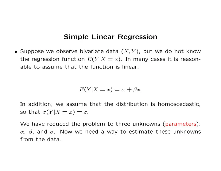
Simple Linear Regression Suppose we observe bivariate data ( X, Y ), - PowerPoint PPT Presentation

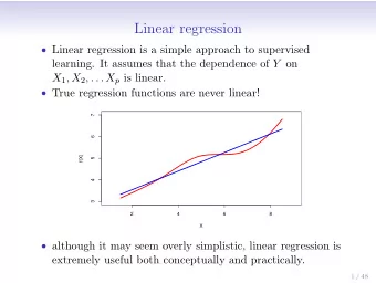
Simple Linear Regression • Suppose we observe bivariate data ( X, Y ), but we do not know the regression function E ( Y | X = x ). In many cases it is reason- able to assume that the function is linear: E ( Y | X = x ) = α + βx. In addition, we assume that the distribution is homoscedastic, so that σ ( Y | X = x ) = σ. We have reduced the problem to three unknowns (parameters): α , β , and σ . Now we need a way to estimate these unknowns from the data.

• For fixed values of α and β (not necessarily the true values), let r i = Y i − α − βX i ( r i is called the residual at X i ). Note that r i is the vertical distance from Y i to the line α + βx . This is illustrated in the following figure: 7 6 5 4 3 2 1 0 -1 -2 -1.5 -1 -0.5 0 0.5 1 1.5 2 A bivariate data set with E ( Y | X = x ) = 3 + 2 X , where the line Y = 2 . 5 + 1 . 5 X is shown in blue. The residuals are the green vertical line segments.

• One approach to estimating the unknowns α and β is to consider the sum of squared residuals function, or SSR. i r 2 i ( Y i − α − βX i ) 2 . When α and The SSR is the function � i = � β are chosen so the fit to the data is good, SSR will be small. If α and β are chosen so the fit to the data is poor, SSR will be large. 8 8 6 6 4 4 2 2 0 0 -2 -2 -4 -4 -6 -6 -8 -8 -10 -10 -2 -1.5 -1 -0.5 0 0.5 1 1.5 2 -2 -1.5 -1 -0.5 0 0.5 1 1.5 2 Left: a poor choice of α and β that give high SSR. Right: α and β that give nearly the smallest possible SSR.

• It is a fact that among all possible α and β , the following values minimize the SSR: ˆ β = cov( X, Y ) / var( X ) Y − ˆ ¯ β ¯ ˆ = α X, These are called the least squares estimates of α and β . The estimated regression function is α + ˆ ˆ E ( Y | X = x ) = ˆ βx and the fitted values are ˆ α + ˆ Y i = ˆ βx i .

• Some properties of the least square estimates: 1. ˆ σ X , so ˆ β = cor( X, Y )ˆ σ Y / ˆ β and cor( X, Y ) always have the same sign – if the data are positively correlated, the es- timated slope is positive, and if the data are negatively correlated, the estimated slope is negative. α + ˆ 2. The fitted line ˆ βx always passes through the overall mean ( ¯ X, ¯ Y ). 3. Since cov( cX, Y ) = c · cov( X, Y ) and var( cX ) = c 2 · var( X ), if we scale the X values by c then the slope is scaled by 1 /c . If we scale the Y values by c then the slope is scaled by c .

α and ˆ • Once we have ˆ β , we can compute the residuals r i based on these estimates, i.e. α − ˆ r i = Y i − ˆ βX i . The following is used to estimate σ : � i r 2 � � � i σ = ˆ n − 2 . �

• It is also possible to formulate this problem in terms of a model, which is a complete description of the distribution that generated the data. The model for linear regression is written: Y i = α + βX i + ǫ i , where α and β are the population regression coefficients, and the ǫ i are iid random variables with mean 0 and standard deviation σ . The ǫ i are called errors.

• Model assumptions: 1. The means all fall on the line α + βX . 2. The ǫ i are iid (no heteroscedasticity). 3. The ǫ i have a normal distribution. Assumption 3 is not always necessary. Least squares estimates α and ˆ ˆ β are still valid when the ǫ i are not normal (as long as 1 and 2 are met). However hypothesis tests, CI’s, and PI’s (derived below) depend on normality of the ǫ i .

α and ˆ • Since ˆ β are functions of the data, which is random, they are random variables, and hence they have a distribution. This distribution reflects the sampling variation that causes ˆ α and ˆ β to differ somewhat from the population values α and β . The sampling variation is less if the sample size n is large, and if the error standard deviation σ is small. The sampling variation of ˆ β is less if the X i values are more variable. We will derive formulas later. For now, we can look at his- tograms.

300 300 250 250 200 200 150 150 100 100 50 50 0 0 0 0.5 1 1.5 2 -3 -2.5 -2 -1.5 -1 α (left) and ˆ Sampling variation of ˆ β (right) for 1000 replicates of the simple linear model Y = 1 − 2 X + ǫ , where SD( ǫ ) = 2 , the sample size is n = 200 , and σ X ≈ 1 . 2 .

250 300 250 200 200 150 150 100 100 50 50 0 0 0 0.5 1 1.5 2 -3 -2.5 -2 -1.5 -1 α (left) and ˆ Sampling variation of ˆ β (right) for 1000 replicates of the simple linear model Y = 1 − 2 X + ǫ , where SD( ǫ ) = 1 / 2 , the sample size is n = 200 , and σ X ≈ 1 . 2 .

300 300 250 250 200 200 150 150 100 100 50 50 0 0 0 0.5 1 1.5 2 -3 -2.5 -2 -1.5 -1 α (left) and ˆ Sampling variation of ˆ β (right) for 1000 replicates of the simple linear model Y = 1 − 2 X + ǫ , where SD( ǫ ) = 2 , the sample size is n = 50 , and σ X ≈ 1 . 2 .

250 250 200 200 150 150 100 100 50 50 0 0 0 0.5 1 1.5 2 -3 -2.5 -2 -1.5 -1 α (left) and ˆ Sampling variation of ˆ β (right) for 1000 replicates of the simple linear model Y = 1 − 2 X + ǫ , where SD( ǫ ) = 2 , the sample size is n = 50 , and σ X ≈ 2 . 2 .

250 250 200 200 150 150 100 100 50 50 0 0 1 1.5 2 2.5 3 1 1.5 2 2.5 3 Sampling variation of ˆ σ for 1000 replicates of the simple linear model Y = 1 − 2 X + ǫ , where SD( ǫ ) = 2 , the sample size is n = 50 (left) and n = 200 (right), and σ X ≈ 1 . 2 .

Sampling properties of the least squares estimates • The following is an identity for the sample covariance: 1 � ( Y i − ¯ Y )( X i − ¯ cov( X, Y ) = X ) n − 1 i 1 n � Y ¯ ¯ = Y i X i − X. n − 1 n − 1 i The average of the products minus the product of the averages (almost).

A similar identity for the sample variance is 1 Y ) 2 ( Y i − ¯ � var( Y ) = n − 1 i 1 n Y 2 Y 2 . � ¯ = i − n − 1 n − 1 i The average of the squares minus the square of the averages (almost).

• An identify for the regression model Y i = α + βX i + ǫ i : 1 1 � � Y i = α + βX i + ǫ i n n i ¯ α + β ¯ Y = X + ¯ ǫ.

• Let’s get the mean and variance of ˆ β : An equivalent way to write the least squares slope estimate is i Y i X i − n ¯ Y ¯ � X ˆ β = X 2 . i X 2 i − n ¯ � Now if we substitute Y i = α + βX i + ǫ i into the above we get i ( α + βX i + ǫ i ) X i − n ( α + β ¯ ǫ ) ¯ X + ¯ X � ˆ β = . i X 2 i − n ¯ X 2 �

Since X 2 � � � � ( α + βX i + ǫ i ) X i = α X i + β i + ǫ i X i i i i X 2 nα ¯ � � = X + β i + ǫ i X i i i we can simplify the expression for ˆ β to get X 2 + � i X 2 i − nβ ¯ ǫ ¯ i ǫ i X i − n ¯ β = β � X ˆ , i X 2 i − n ¯ X 2 � and further to ǫ ¯ i ǫ i X i − n ¯ X � ˆ β = β + i X 2 i − n ¯ X 2 �

To apply this result, by the assumption of the linear model Eǫ i = ǫ = 0, so E cov( X, ǫ ) = 0, and we can conclude that E ˆ E ¯ β = β . This means that ˆ β is an unbiased estimate of β – it is correct on average. If we observe an independent SRS every day for 1000 days from the same linear model, and we calculate ˆ β i each day for i = 1 , . . . , 1000, the daily ˆ β i may differ from the population β due to i ˆ sampling variation, but the average � β i / 1000 will be extremely close to β .

• Now that we know E ˆ β = β , the corresponding analysis for ˆ α is straightforward. Since α = ¯ Y − ˆ β ¯ ˆ X, then α = E ¯ Y − β ¯ E ˆ X, and since ¯ Y = α + β ¯ ǫ , so E ¯ Y = α + β ¯ X + ¯ X , thus α = α + β ¯ X − β ¯ E ˆ X = α, so α is also unbiased.

• Next we would like to calculate the standard deviation of ˆ β , which will allow us to produce a CI for β . Beginning with ǫ ¯ i ǫ i X i − n ¯ � X ˆ β = β + i X 2 i − n ¯ X 2 � and applying the identity var( U − V ) = var( U )+var( V ) − 2cov( U, V ): ǫ ¯ ǫ ¯ β ) = var( � i ǫ i X i ) + var( n ¯ X ) − 2cov( � i ǫ i X i , n ¯ X ) var(ˆ . i X 2 i − n ¯ X 2 ) 2 ( � Simplifying i var( ǫ i ) + n 2 ¯ i X 2 X 2 var(¯ ǫ ) − 2 n ¯ i X i cov( ǫ i , ¯ ǫ ) � X � var(ˆ β ) = . i X 2 i − n ¯ X 2 ) 2 ( �

Next, using var( ǫ i ) = σ 2 , var(¯ ǫ ) = σ 2 /n : i + nσ 2 ¯ X 2 − 2 n ¯ β ) = σ 2 � i X 2 X � i X i cov( ǫ i , ¯ ǫ ) var(ˆ . i X 2 i − n ¯ X 2 ) 2 ( � � cov( ǫ i , ¯ ǫ ) = cov( ǫ i , ǫ j ) /n j σ 2 /n. = So we get i + nσ 2 ¯ X 2 − 2 n ¯ σ 2 � i X 2 i X i σ 2 /n X � var(ˆ β ) = i X 2 i − n ¯ X 2 ) 2 ( � i + nσ 2 ¯ X 2 − 2 n ¯ σ 2 � i X 2 X 2 σ 2 = . i X 2 i − n ¯ X 2 ) 2 ( �

Alomst done: σ 2 � i X 2 X 2 σ 2 i − n ¯ var(ˆ β ) = i X 2 i − n ¯ X 2 ) 2 ( � σ 2 = i X 2 i − n ¯ X 2 � σ 2 = ( n − 1)var( X ) , and σ sd(ˆ β ) = √ n − 1ˆ . σ X

• The slope SD formula is consistent with the three factors that influenced the precision of ˆ β in the histograms: 1. greater sample size reduces the SD 2. greater σ 2 increases the SD 3. greater X variability (ˆ σ X ) reduces the SD.

• A similar analysis for ˆ α yields � X 2 i /n α ) = σ 2 var(ˆ ( n − 1)var( X ) . β ) � X 2 α ) = var(ˆ Thus var(ˆ i /n . Due to the � X 2 i /n term the estimate will be more precise when the X i values are close to zero. Since ˆ α is the intercept, it’s easier to estimate when the data is close to the origin.