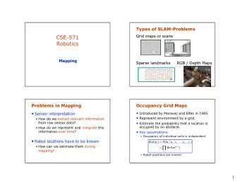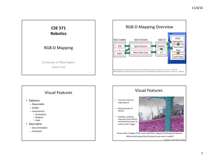
RGB-D Mapping Overview CSE 571 Robotics Map RGB-D Mapping `` - PowerPoint PPT Presentation

11/6/16 RGB-D Mapping Overview CSE 571 Robotics Map RGB-D Mapping `` University of Washington Dieter Fox RGB-D Mapping: Using Depth Cameras for Dense 3D Modeling of Indoor Environments. Henry et al. ISER 2010 RGB-D Mapping: Using Kinect-style Depth Cameras for Dense 3D Modeling of Indoor Environments. Henry et al. IJRR 2012 1 2 Visual Features Visual Features • Detector • Tree bark itself not really distinct – Repeatable – Stable • Rocky ground not – Invariances: distinct • Illumination • Rooftops, windows, • Rotation lamp post fairly distinct • Scale and should be easier to • Descriptor match across images – Discriminative – Invariant Say we have 2 images of this scene we’d like to align by matching local features What would be good local features (ones easy to match)? 3 Courtesy: S. Seitz and R. Szeliski 1

11/6/16 Scale Invariant Feature Transform Invariant local features -Algorithm for finding points and representing their patches should produce Basic idea: similar results even when conditions vary • Take 16x16 square window around detected feature -Buzzword is “invariance” • Compute gradient for each pixel – geometric invariance: translation, rotation, scale • Throw out weak gradient magnitudes – photometric invariance: brightness, exposure, … • Create histogram of surviving gradient orientations 0 2 p angle histogram Feature Descriptors Adapted from slide by David Lowe Courtesy: S. Seitz and R. Szeliski SIFT keypoint descriptor Properties of SIFT Extraordinarily robust matching technique Full version – Can handle changes in viewpoint • Divide the 16x16 window into a 4x4 grid of cells (2x2 case shown below) • Up to about 60 degree out of plane rotation • Compute an orientation histogram for each cell – Can handle significant changes in illumination • 16 cells * 8 orientations = 128 dimensional descriptor • Sometimes even day vs. night (below) – Fast and efficient—can run in real time – Lots of code available • http://www.vlfeat.org • http://www.cs.unc.edu/~ccwu/siftgpu/ Adapted from slide by David Lowe 2

11/6/16 Feature distance Feature distance • How to define the difference between two features f1, f2? • How to define the difference between two features f1, f2? – Simple approach is SSD(f1, f2) – Better approach: ratio distance = SSD(f1, f2) / SSD(f1, f2’) • sum of square differences between entries of the two descriptors • f2 is best SSD match to f1 in I 2 • can give good scores to very ambiguous (bad) matches • f2’ is 2nd best SSD match to f1 in I 2 • gives small values for ambiguous matches f 1 f 2 f 1 f 2' f 2 I 1 I 2 I 1 I 2 Are descriptors unique? Are descriptors unique? No, they can be matched to wrong features, generating outliers. 11 12 3

11/6/16 Strategy: RANSAC Simple Example • RANSAC loop: • Fitting a straight line 1. Randomly select a seed group of matches 2. Compute transformation from seed group 3. Find inliers to this transformation 4. If the number of inliers is sufficiently large, re-compute least-squares estimate of transformation on all of the inliers • Keep the transformation with the largest number of inliers M. A. Fischler, R. C. Bolles. Random Sample Consensus: A Paradigm for Model Fitting with Applications to Image Analysis and Automated Cartography. Comm. of the ACM, Vol 24, pp 381-395, 1981. RANSAC example: Translation Why will this work ? Putative matches Slide: A. Efros 4

11/6/16 RANSAC example: Translation RANSAC example: Translation Select one match, count inliers Find “average” translation vector Slide: A. Efros Slide: A. Efros RANSAC: Line Fitting RANSAC pros and cons • Pros – Simple and general – Applicable to many different problems – Often works well in practice • Cons – Lots of parameters to tune – Can’t always get a good initialization of the model based on the minimum number of samples – Sometimes too many iterations are required – Can fail for extremely low inlier ratios 5

11/6/16 Visual Odometry Visual Odometry Failure Cases • Compute the motion between consecutive camera frames from visual feature correspondences. • Low light, lack of visual texture or features • Visual features from RGB image have a 3D counterpart • Poor distribution of features across image from depth image. • But: RGB-D camera still provides shape info • Three 3D-3D correspondences constrain the motion. 21 22 ICP ICP Variants (Iterative Closest Point) • Iterative Closest Point (ICP) uses shape to align • Correspondence frames – Outliers as absolute or percentage • Does not require the RGB image – No many-to-one correspondences – Reject boundary points • Does need a good initial “guess” – Normal agreement • Repeat the following two steps: • Error metric – For each point in cloud A, find the closest corresponding point in cloud B – Point-to-point – Point-to-plane – Compute the transformation that best aligns this set of corresponding pairs – Weight by color / normal agreement 23 24 6

11/6/16 ICP (Iterative Closest Point) ICP Failure Cases • Iteratively align frames based on shape • Not enough distinctive shape • Needs a good initial estimate of the pose • Don’t have a close enough initial “guess” • Here the shape is basically a simple plane… 25 26 Optimal Transformation Joint Optimization (RGBD-ICP) • Jointly minimize feature re-projection and ICP: RGB-D Mapping: Using Depth Cameras for Dense 3D Modeling of Indoor Environments. Henry et al. ISER 2010 RGB-D Mapping: Using Kinect-style Depth Cameras for Dense 3D Modeling of Indoor Environments. Henry et al. IJRR 2012 27 28 7

11/6/16 Loop Closure Experiments • Sequential alignments accumulate error • Reprojection error is better for RANSAC: • Revisiting a previous location results in an inconsistent map • Errors for variations of the algorithm: • Timing for variations of the algorithm: 29 30 Loop Closure Detection • Detect by running RANSAC against previous frames • Pre-filter options (for efficiency): – Only a subset of frames ( keyframes ) – Only keyframes with similar estimated 3D pose – Place recognition using vocabulary tree • Scalable recognition with a vocabulary tree , David Nister and Henrik Stewenius, 2006 • Post-filter (avoid false positives) – Estimate maximum expected drift and reject detections changing pose too greatly 31 32 8

11/6/16 [Image: Manolis Lourakis] Loop Closure Correction: Loop Closure Correction (TORO) Bundle Adjustment • TORO [Grisetti 2007, 2009]: – Constraints between camera locations in pose graph – Maximum likelihood global camera poses 33 34 SBA Points 35 36 9

11/6/16 A Second Comparison Timing TORO SBA 37 38 Resulting Map 39 40 10

11/6/16 Experiments: Overlay 1 Experiments: Overlay 2 41 42 Map Representation: Surfels • Surface Elements [Pfister 2000, Weise 2009, Krainin 2010] • Circular surface patches • Accumulate color / orientation / size information • Incremental, independent updates • Incorporate occlusion reasoning • 750 million points reduced to 9 million surfels 43 44 11

11/6/16 Application: Quadrocopter • Collaboration with Albert Huang, Abe Bacharach, and Nicholas Roy from MIT 45 46 Larger Maps 47 12

11/6/16 [Whelan-Leutenegger-SalasMoreno-Glocker-Davison: RSS-15] ElasticFusion 50 Conclusion • Kinect-style depth cameras have recently become available as consumer products • RGB-D Mapping can generate rich 3D maps using these cameras • RGBD-ICP combines visual and shape information for robust frame-to-frame alignment • Global consistency achieved via loop closure detection and optimization (RANSAC, TORO, SBA) • Surfels provide a compact map representation 51 13